Teacher’s Guide for Geometry: Seeing, Doing, Understanding

Complete conversion in a single file. See README.md for the version split by chapter.

Introduction: Euclid, the Surfer and the Spotter

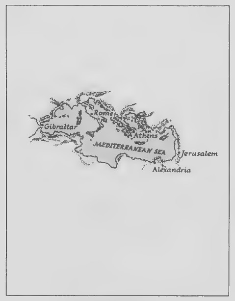Transparency 0-1: Map around the Mediterranean

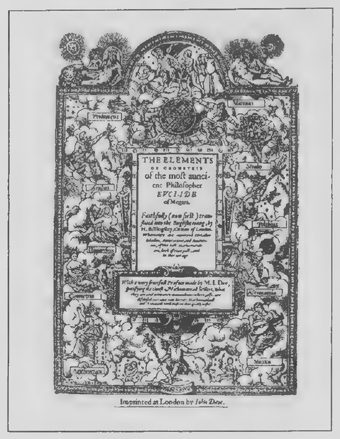Transparency 0-2: Title page of Euclid’s Elements

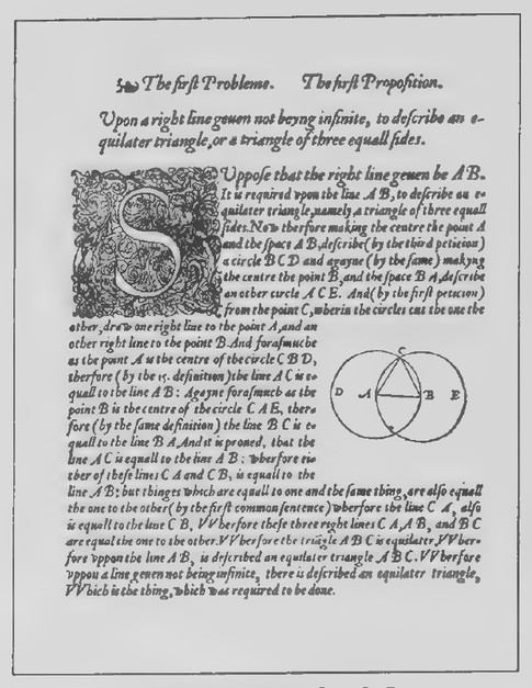Transparency 0-3: Proposition 1 from the Elements

Introduction: Euclid, the Surfer and the Spotter

Transparencies

• 0-1 Map around the Mediterranean
• 0-2 Title page of Euclid’s Elements
• 0-3 Proposition 1 from the Elements
• 0-4 The surfer and the spotter
• 0-5 The spotter’s puzzle
• 0-6 The surfer’s puzzle

The introductory section includes a brief commentary on Euclid and the Elements, the construction of an equilateral triangle, and the puzzles of the surfer and the spotter. Although this material could be assigned as homework, I recommend doing and discussing it in class. You will probably need to provide your students with rulers and compasses.

The puzzle of the spotter is to find the location of the point inside or on an equilateral triangle for which the sum of the distances from that point to the vertices of the triangles is a minimum. After some experimentation, your students should conclude that this point is at the “center” of the triangle. The three paths from the center to the vertices would have the same length: their sum is about 20.8 km. The worst place on the island for the spotter to locate is at the point for which the sum of its distances to the vertices of the triangle is a maximum. There are actually three of these points—namely, the vertices themselves. The sum of the lengths of the paths from one vertex to the other two is 24.0 km.

The surfer’s puzzle consists of trying to find the

location of the point inside or on an equilateral triangle for which the sum of the distances from that point to the sides of the triangle is a minimum. Before they try any points, your students will probably assume that the answer to this puzzle is the same as before. It is a remarkable fact, however, that the sum of the three distances is the same for every point either inside or on the triangle! It is about 10.4 km. Hence, there is no best or worst place for the surfer to locate.

My students are generally content with their analysis of the spotter’s puzzle. Although they haven’t proved why the center is the best place and the corners are the worst, these answers seem reasonable.

The result of the surfer’s puzzle, on the other hand, is surprising and hence disconcerting. Why should the sum of the three distances be independent of the position of the point? Certainly no amount of experimentation is capable of either proving or explaining this claim. This realization suggests that, to be confident of the conclusions that we may draw in geometry, we must have some basis for understanding them and for convincing others that they are correct. Deductive reasoning provides this basis, and it is the subject of the second chapter of the course.

Transparencies 0-1 through 0-4 are for use in presenting the introductory lesson. Transparencies 0-5 and 0-6 and their overlays illustrate many dif-

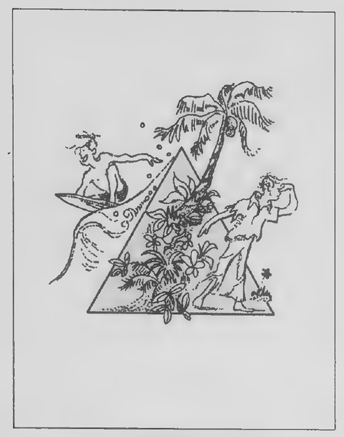Transparency 0-4: The surfer and the spotter

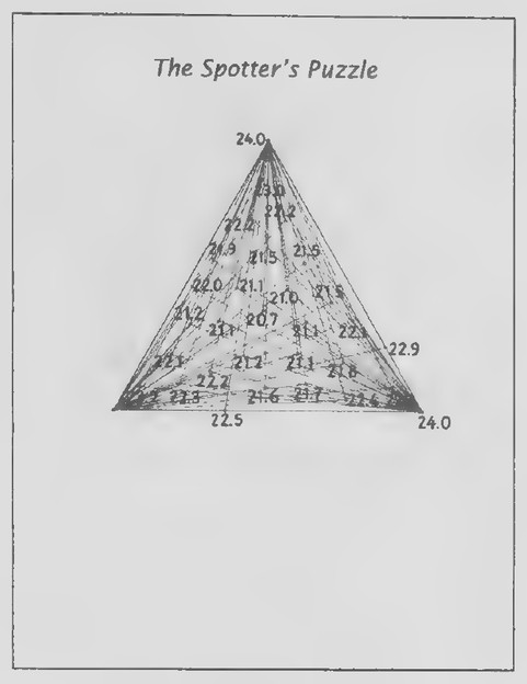Transparency 0-5: The spotter’s puzzle

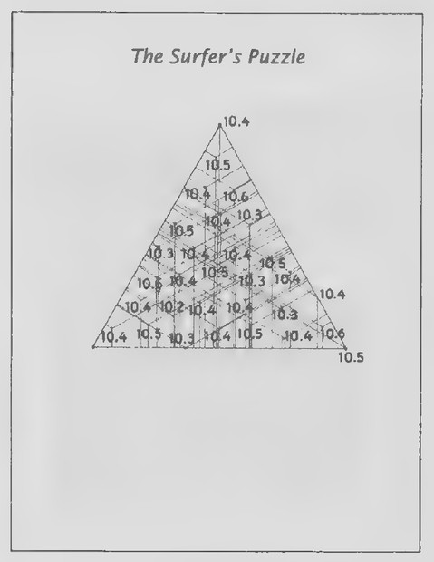Transparency 0-6: The surfer’s puzzle

ferent points for each puzzle and the distance sums that correspond to the points.

The spotter’s puzzle is a special case of a problem proposed by Pierre Fermat; its solution is based on the fact that the perpendicular segment from a point to a line is the shortest segment connecting them. The solution to the surfer’s puzzle can be understood by means of the theory of area. Both puzzles will be reconsidered later in the course.*

*An explanation of the surfer’s puzzle is developed in Chapter 9, Lesson 3, exercises 29-34 of the text. The spotter’s, puzzle is discussed in the second review lesson for Chapter 13 of the Teacher’s Guide.

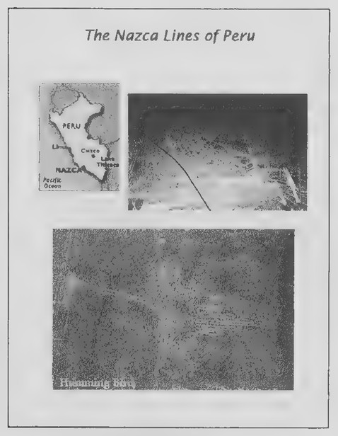Transparency 1-1-1: The Nazca lines of Peru

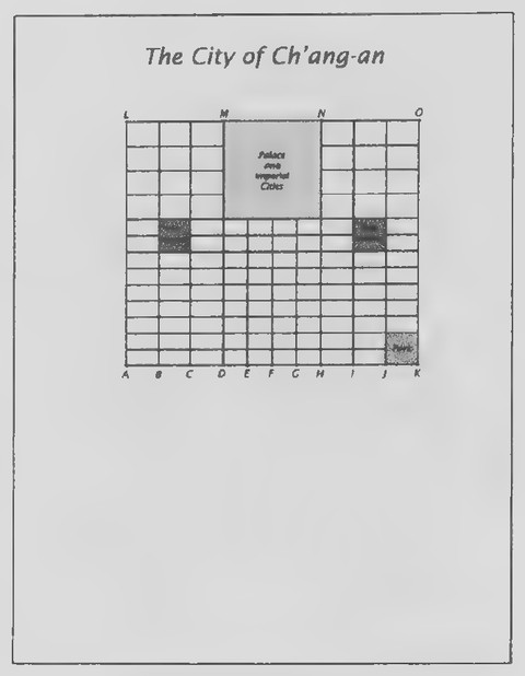Transparency 1-1-2: The city of Ch’ang-an (Set I)

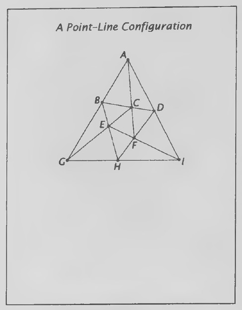Transparency 1-1-3: A point-line configuration (Set II)

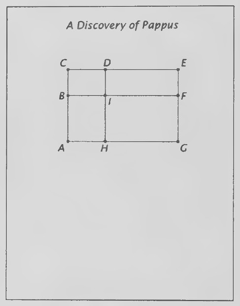Transparency 1-1-4: A discovery of Pappus (Set III)

Chapter 1: An Introduction to Geometry

Lesson 1: Lines in Designing a City

Lesson Outline

Terms: Point, line, line segment, plane, collinear, noncollinear, coplanar, concurrent.

Transparencies

• 1-1-1 The Nazca lines of Peru
• 1-1-2 The city of Ch’ang-an (Set I)
• 1-1-3 A point-line configuration (Set II)
• 1-1-4 A discovery of Pappus (Set III)

Introduction

One of the world’s unsolved mysteries concerns the desert of southern Peru. Stretching for miles across the land are gigantic drawings of birds and other animals, as well as lines—many lines—leading in every direction. The drawings and lines were put there by the Nazca civilization more than 1,500 years ago. For what purpose, no one knows.

Strange as it may seem, the people who drew these figures probably never saw them in their entirety, because they can only be seen from heights of at least 1,000 feet. They weren’t noticed until the 1920s when airplanes began flying over the Peruvian desert.*

Some of the lines extend for many miles and are incredibly straight. The Nazcas are thought to have stretched strings from posts to aid in their construction. How many posts would be needed to determine the direction of one of these strings? (Two.) The positions of the posts are good models of geometric points, and the stretched string is a good model of part of a geometric line. The flatness of the Nazca plain on which the figures were created makes it a good model of a geometric plane.

This introduction leads naturally into the rest of the ideas included in the lesson. Guide your students in listing and making sketches illustrating the basic terms before they begin the exercises.

*Further information about the Nazca (also spelled Nasca) lines can be found in Pathways to the Gods, by Tony Morrison (Harper & Row, 1978), The World’s Last Mysteries (A Reader’s Digest Book, 1978), and various sites on the Internet, including www.crystalinks.com/nasca.html.

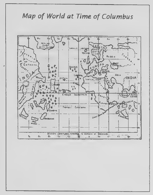Transparency 1-2-1: Map of world at time of Columbus

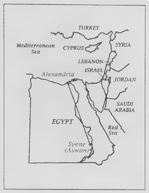Transparency 1-2-2: Map of Alexandria and Syene

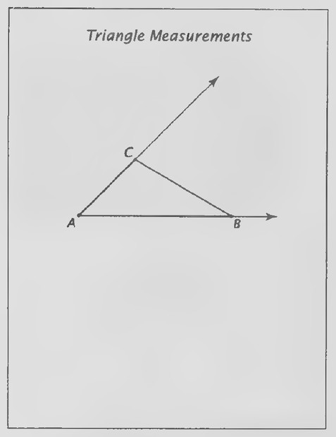Transparency 1-2-3: Triangle measurements (Set I, Exs. 1-12)

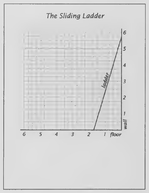Transparency 1-2-4: The sliding ladder (Set II)

Lesson 2: Angles in Measuring the Earth

Lesson Outline

Terms: Ray, angle (sides and vertex), protractor, degree.

Transparencies

• 1-2-1 Map of world at time of Columbus
• 1-2-2 Map of Alexandria and Syene
• 1-2-3 Triangle measurements (Set I, Exs. 1-12)
• 1-2-4 The sliding ladder (Set II)

Introduction

Good opening questions: Do you know what the distance around the earth is? How long ago do you suppose it was first determined?

In the foreword to the book titled The Log of Christopher Columbus, edited by Robert H. Fuson (International Marine Publishing Company, 1987), Luis Marden wrote:

“No literate person in 1492 thought the world was flat; the Greeks had proved the sphericity of the earth long before Christ. In fact, in that same year of 1492 Martin Behaim in Germany produced a terrestrial globe, still extant. The question under debate was the size of the globe. In the third century B.C., the Greek astronomer Eratosthenes, using only his brain and a shadow-casting column, came astonishingly close to the true circumference, but 500 years later the geographer Ptolemy described an earth one fourth smaller than the true dimension.”

Columbus thought that the circumference of the earth was approximately 20,000 miles. If he had known the correct value, he might not have at-

tempted the journey. As Fuson remarks, Columbus’s belief that the earth was much smaller than it is “was one of the most fortunate mistakes in history.”

The map on Transparency 1-2-1, based on Behaim’s world globe of 1492, makes clear why when he sailed west from Spain and arrived at Cuba, Columbus thought it was Japan (Cipango). Not until considerably later did the Europeans realize that the earth was large enough to contain another continent and ocean.

How could someone have accurately determined the size of the earth more than seventeen centuries before Columbus made his historic voyage? Explain the method that Eratosthenes used as described on pages 14 and 15 of the text by first showing Transparency 1-2-2 and then having your

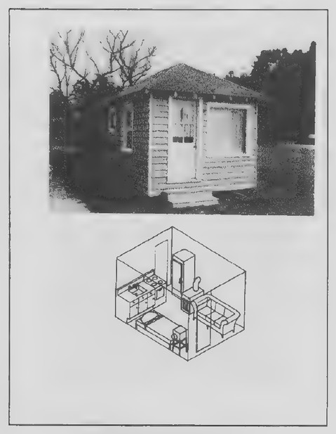Transparency 1-3-1: Tiny house

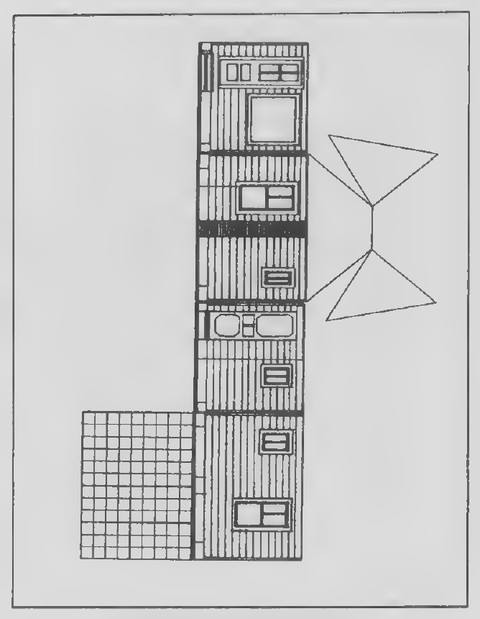TINY HOUSE PATTERN

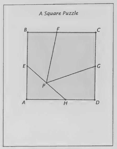Transparency 1-3-2: A square puzzle (Set III)

students draw the following figure. Use the semicircular edge of a protractor to draw a circle to represent the earth. Mark a point, S, at the top of the circle to represent Syene and draw a ray upward from the center of the circle through this point to show the direction of the sun when it is directly overhead. Use the protractor to draw an angle with this ray as one of its sides and with a measure of 7.5° to find the position, A, of Alexandria on the circle. Draw a ray from point A parallel to the original ray to complete the figure and then guide your students in discovering what Eratosthenes did.

Lesson 3: Polygons and Polyhedra: Pyramid Architecture

Lesson Outline

Terms: Polygon (triangle, quadrilateral, pentagon, hexagon, octagon), polyhedron, perimeter, area, rectangle, square.

Transparencies and Worksheet

• 1-3-1 Tiny house Tiny house pattern
• 1-3-2 Asquare puzzle (Set III) (Cut out a set of the four pieces for use in illustrating how they can be rearranged to form the equilateral triangle.)

Introduction

Before class, tape off a rectangle measuring 9 ft by 12 ft on the floor of your classroom to illustrate just how small the tiny house featured in this lesson actually is. The house is located near Whitestone, Virginia. Designed as a 1950s ranch house, it consists of just one room 12 ft long and 9 ft wide. Its interior

is shown in the diagram below the photograph. (Its bathroom is a separate outhouse, not visible in the picture.)*

Hand out scissors and copies of the Tiny House Pattern so that your students can put together a simple model of the house. Before they do so, observe that the figures representing the walls, floor, and sections of the roof are examples of polygons [triangles and quadrilaterals (rectangles, squares, and trapezoids)|. The surfaces of the house, after it has been put together, provide an example of a polyhedron (one having nine faces). If the pattern is cut out as a single piece and just one piece of tape used to connect the unattached walls, it can be folded flat again after the lesson has been completed. The rectangle representing the floor of the house has been divided into small squares, each corresponding to 1 square foot. The model can thus be used to develop the rest of the lesson by having your students consider the perimeter and area of the floor.

Lesson 4: Constructions: Telling Time with Shadows

Lesson Outline

Terms: Straightedge, compass, circle (radius, center), construction, bisect.

Constructions: To bisect a line segment, to bisect an angle.

Transparencies

• 1-4-1 Counterclockwise clock
• 1-4-2 Sundial

*Tiny Houses, by Lester Walker (Overlook Press, 1987).

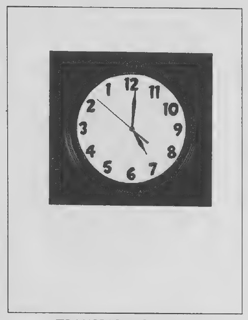Transparency 1-4-1: Counterclockwise clock

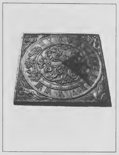Transparency 1-4-2: Sundial

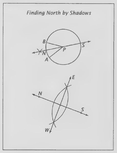Transparency 1-4-3: Finding North by Shadows

1-4-3. Finding north by shadows (Set I, Exs. 3-9) 1-4-4 Bisectors in a triangle (Set I, Exs. 10-16)

Introduction

An amusing way to begin this lesson is to have a “backward clock” in view in your classroom as your students arrive. Such clocks are available for about $15 from many different sources on the Internet and can be found by typing “backward clock” on your search engine. The clock shown on Transparency 1- 4-1 is an example of one of these clocks. Ask your students how a clock with its numbers in reverse order could keep correct time. (Its hands go counterclockwise.) The manufacturer of one of these clocks states: “Does the frantic pace of today’s world make you want to turn back the hands of time and give yourself a few extra hours? We’ve solved this problem for you with our new Backward Clock. The hour, minute and second hands move backward to give you the extra time you need. The numbers on this clock are arranged counterclockwise to help you keep track of how much time you’re saving.”

Why do clocks ordinarily run “clockwise”? In his book titled Why Do Clocks Run Clockwise? and Other Imponderables (Harper & Row, 1987), David Feldman gives the following explanation: “Before the advent of clocks, we used sundials. In the northern hemisphere, the shadows rotated in the direction we now call ‘clockwise.’ The clock hands were built to mimic the natural movement of the sun. If clocks had been invented in the southern hemisphere… ‘clockwise’ would be the opposite direction.” The sundial pictured on Transparency 1-4-2 illustrates this resemblance nicely. In their book on

Time (Life Science Library, 1980), Samuel A. Goudsmit and Robert Claiborne observe: “As long as the principal timekeeper was the motion of the sun—for some 4,000 years from ancient Egypt to the 16th Century—the main timekeeping device was the sundial…. The sundial is remarkably reliable, so good that for centuries it was employed to correct mechanical clocks.”

Have your students use a compass to draw a circle and a horizontal diameter. Show them how to construct a vertical diameter and label the endpoints of the diameters according to map directions with north at top. Point out that their drawing lies in the horizontal plane of the paper. Imagine a vertical post with its base at the center of the circle. In what direction would its shadow point when the sun is rising in the east? (West.) Where is the sun in the sky at noon? (In the Northern Hemisphere, it is toward the south.) In what direction does the shadow of the post point at noon? (North.) In what direction does the shadow point when the sun is setting in the west? (East.) The answers to these questions confirm the fact that, in the Northern Hemisphere, shadows turn clockwise during the day.

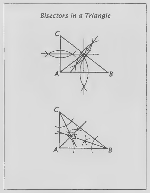Transparency 1-4-4: Bisectors in a triangle (Set I, Exs. 10-16)

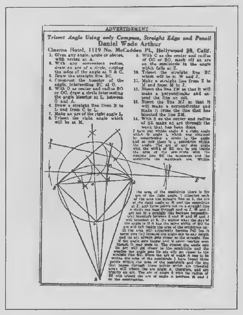Transparency 1-5-1: Angle-trisection advertisement

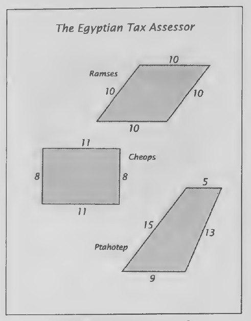Transparency 1-5-2: The Egyptian tax assessor

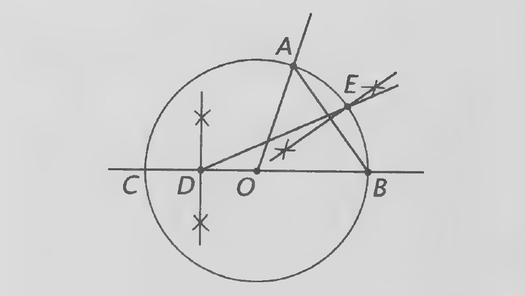Figure on page 296 — Compass-and-straightedge angle-bisection construction: a circle with center O cut by rays to A and B, with arc marks on OC and the line DE

Lesson 5: We Can’t Go On Like This

Lesson Outline

Theme: The need to know why.

Transparencies

• 1-5-1 Angle-trisection advertisement
• 1-5-2 The Egyptian tax assessor

Introduction

[This introduction is especially appropriate in that it both reviews the bisection constructions of Lesson 4 and leads naturally into the new lesson.] A very strange advertisement (Transparency 1-5-1) once appeared in the Los Angeles Times. It was paid for by a man named Daniel Wade Arthur whose address was a cheap hotel in Hollywood. The ad appeared in the Sunday paper and was rather large; so Mr. Arthur had to have paid a lot of money to run it. He didn’t have any hope of making any money from it, because he wasn’t trying to sell anything. The subject of the ad was a geometry problem! Mr. Arthur was explaining how to trisect an angle using only a compass, straightedge, and pencil. His method was very complicated and would take a lot of time and effort to carry out, which makes one wonder if anyone who saw the ad in the paper bothered to even read it.

A French mathematician published a much simpler way to “trisect an angle” in 1934.* To try it out,

have your draw an angle of 72° and then carry out the construction as illustrated in the figure above and described in the following steps:

1. Draw a circle with its center at the vertex of the

angle, O, and let A and B be the points in which

it intersects the sides of the angle. 2. Extend line OB to intersect the circle at C. 3. Bisect CO and let D be its midpoint. 4. Draw AB, bisect it and let E be the point in which

the bisecting line intersects the circle. 5. Draw line DE.

∠EDB appears to have a measure of 24°, and so ∠AOB appears to have been trisected. However, if ∠AOB is exactly 72°, then it can be proved that ∠EDB has a measure of slightly more than 24°. So the method doesn’t quite work, but the mathematician who thought of it realized this. He knew that another mathematician had proved sucha construction to be impossible in 1837, almost a hundred years earlier. Unfortunately for Mr. Arthur, the man who

*The mathematician, Maurice d’Ocagne (1862-1938), was sufficiently famous in France that a street in Paris is now named for him. For an approximation, his method is especially accurate for angles less than 20°. An analysis of it can be found on page 55 of The Trisection Problem, by Robert C. Yates (Franklin Press, 1942; reprinted by N.C.T.M., 1971).

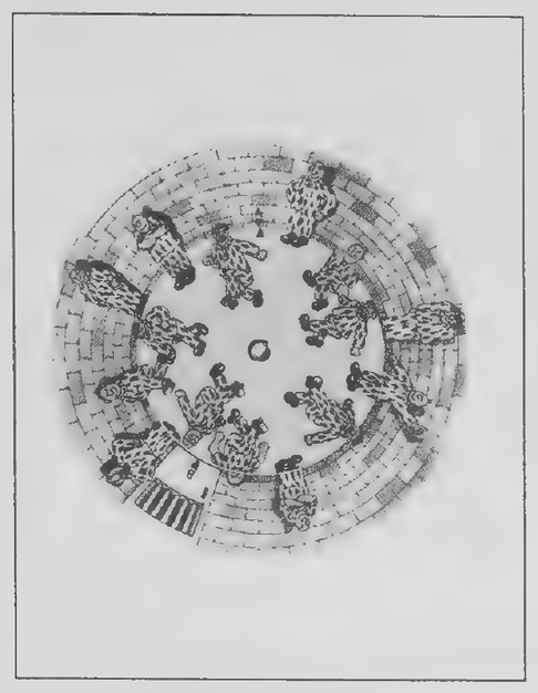Transparency 1-R-1: Find the escapee

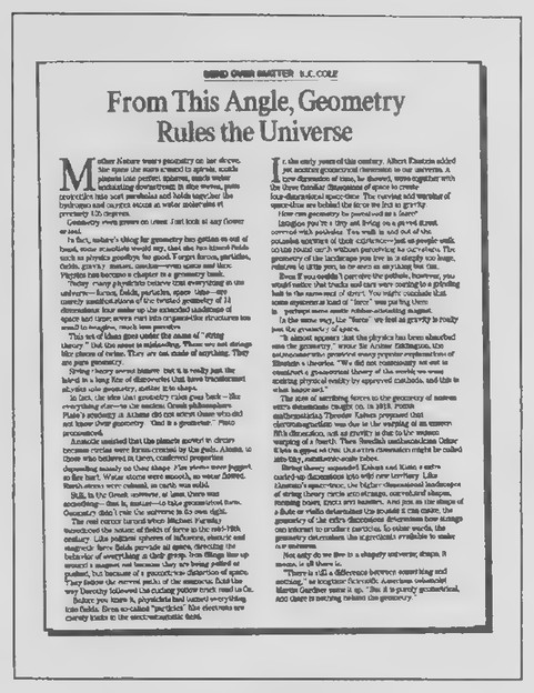Transparency 1-R-2: Geometry rules the universe

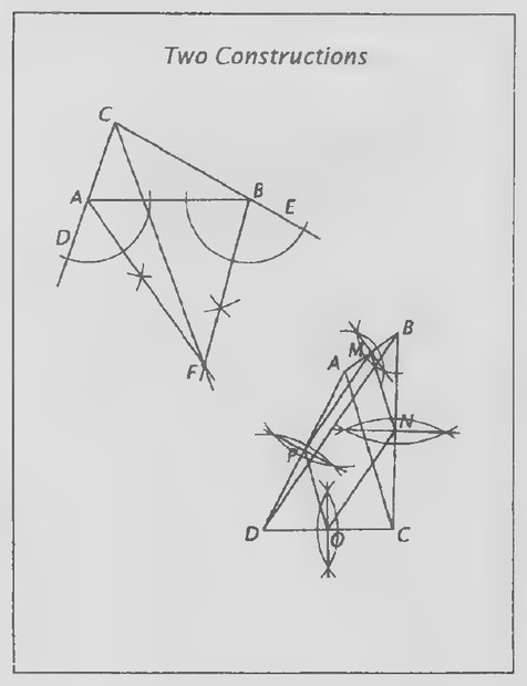Transparency 1-R-3: Two constructions (Set II)

spent his money on the angle trisection ad, this means that his method doesn’t quite work either. If his method had worked, his money would have been well spent because his name would have become famous in the history of mathematics for succeeding in doing something that people have been trying to figure out ever since the time of Euclid.

The situation presented by the problem of trisecting an angle with just a straightedge and compass leads naturally to several questions. How do you prove that something is impossible? How is it possible to tell the difference between exactly right and almost? How do you prove something in the first place? To eventually be able to answer such questions is a major goal of the study of geometry.

Students who would like to know more about the problem of angle trisection and how people have tried to solve it may be interested in reading the chapter titled “How to Trisect an Angle” in Mathematical Carnival, by Martin Gardner (Knopf, 1975) and looking through A Budget of Trisections, by Underwood Dudley (Springer Verlag, 1987).

Review of Chapter 1

First day

Transparencies

• 1-R-1 Find the escapee
• 1-R-2 Geometry rules the universe
• 1-R-3 Two constructions (Set II)
• 1-R-4 Russian second-grade problem

Introduction

A light-hearted way to begin the review lesson is with a “Geometrical Vanish.” In his book titled

Mathematics, Magic and Mystery (Dover, 1956), Martin Gardner includes two chapters on puzzles of this sort. He describes these puzzles as geometrical paradoxes that consist of “rearranging parts of a figure. After the rearrangement is completed, a portion of the original figure (either part of its area or one of a series of pictures drawn on the figure) has apparently vanished without trace. When the pieces are returned to their original form, the missing area or picture mysteriously appears once more.” American puzzlist Sam Loyd invented and patented an extremely clever puzzle of this sort in 1896. Called “Get Off the Earth,” more than 10 million copies of it were sold in Loyd’s lifetime.

Australian physicist Dugald Keith was inspired by Loyd’s puzzle to create a puzzle with the title “Find the Escapee.” Pictured on Transparency 1-R- 1 and its overlay, the puzzle shows 15 prisoners ina circular jail cell when the arrow on the overlay points to A; when the overlay is turned so that the arrow points to B, one of the prisoners has vanished.

Alternative Introduction A recent article in the Los Angeles Times (Transparency 1-R-2) claims that “Geometry Rules the Universe.” Although it would not be appropriate to read it to your class in its entirety, your students may find the following excerpts to be of interest (italics added for emphasis):

“Mother Nature wears geometry on her sleeve. She spins the stars around in spirals, molds planets into perfect spheres, sends water undulating downstream in sine waves, pulls projectiles into neat parabolas and holds together the hydrogen and oxy-

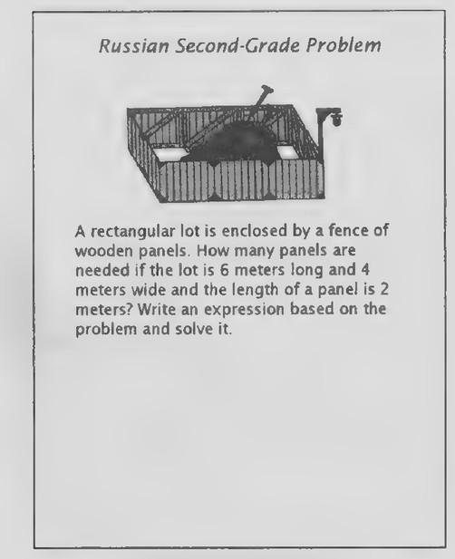Transparency 1-R-4: Russian second-grade problem

gen atoms in water molecules at precisely 105 degrees.

Geometry even grows on trees: Just look at any flower or leaf.

In fact, nature’s thing for geometry has gotten so out of hand, some scientists would say, that she has kissed fields such as physics goodbye for good. Forget forces, particles, fields, gravity, matter, motion—even space and time. Physics has become a chapter in a geometry book.

Today, many physicists believe that everything in the universe—forces, fields, particles, space, time—are merely manifestations of the twisted geometry of 11 dimensions: four make up the extended landscape of space and time; seven curl into origami-like structures too small to imagine, much less perceive.

This set of ideas goes under the name of ‘string theory.’ But the name is misleading. These are not strings like pieces of twine. They are not made of anything. They are pure geometry.

String theory seems bizarre, but it is really just the latest in a long line of discoveries that have transformed physics into geometry, matter into shape.

In fact, the idea that geometry rules goes back—like everything else—to the ancient Greek philosophers. Plato’s academy in Athens did not admit those who did not know their geometry. ‘God is a geometer,’ Plato pronounced.”

[The article goes on to describe Faraday’s introduction of the idea of force fields, geometrical distortions of space, in the nineteenth century; Einstein’s addition of another geometrical dimension, time, in the twentieth century to form four-

dimensional space-time, used to explain gravity; and the use of string theory to explain why elementary particles exist.]

“In other words,… geometry determines the ingredients available to make our universe.

Not only do we lie ina shapely universe; shape, it seems, is all there is.

‘There is still a difference between something and nothing,’ as longtime Scientific American columnist Martin Gardner sums it up. ‘But it is purely geometrical, and there is nothing behind the geometry.”

Second day

Introduction

People immigrating to the United States are sometimes surprised at the difference between what was taught in their former countries and what their children encounter in their new country. Here is an example that may surprise you. This problem (Transparency 1-R-4) appeared in a book for second-graders used for many years throughout the former Soviet Union. What expression do you think the students were expected to write? What is the solution

6+4+6+4 2(6 + 4) to the problem? ( eer ea; 10 pan-

2 Slik? els.) Suppose that the problem were stated in terms of variables rather than numbers: How many panels are needed if the lot is x m long and y m wide and

the length of a panel is z m² (F2h) In writing

this expression, what are we assuming about z, the length of a panel, with respect to x and y, the dimensions of the lot? (That z divides evenly into x and y.) These more general questions will suggest to some of your students the need for some review of algebra. The first algebra review appears at the end of this chapter and might be done in class as time allows after the chapter review has been completed.

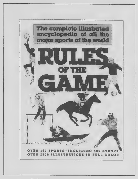Transparency 2-1-1: Rules of the Game book cover

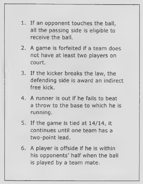Transparency 2-1-2: Rules that are conditional statements

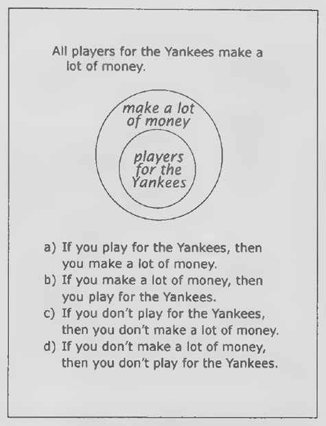Transparency 2-1-3: Yankees problems (Set II, Exs. 31-33)

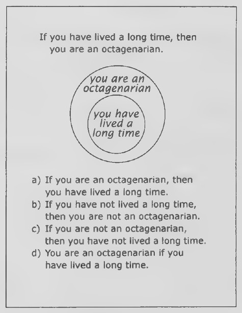Transparency 2-1-4: Octagenarian problems (Set II, Exs. 34-36)

Chapter 2: The Nature of Deductive Reasoning

Lesson 1: Conditional Statements

Lesson Outline

Terms: Conditional statement (hypothesis, conclusion), Euler diagram.

Transparencies

• 2-1-1 Rules of the Game book cover
• 2-1-2 Rules that are conditional statements
• 2-1-3 Yankees problems (Set II, Exs. 31-33)
• 2-1-4 Octagenarian problems (Set II, Exs. 34-36)

Introduction

Show Transparencies 2-1-1 and 2-1-2. Every game is played by rules. Here are some examples of rules for various sports that are listed in a book titled Rules of the Game (The Diagram Group, St. Martin’s Press, 1990). Which sports can you identify?

1. If an opponent touches the ball, all the

passing side is eligible to receive the ball.

(Football.)

2. A game is forfeited if a team does not have

at least two players on court. (Basketball.)

3. If the kicker breaks the law, the defending

side is awarded an indirect free kick.

(Soccer.)

4. Arunner is out if he fails to beat a throw to

the base to which he is running. (Baseball.)

5. If the game is tied at 14/14, it continues

until one team has a two-point lead.

(Volleyball.)

6. A player is offside if he is within his oppo-

nents’ half when the ball is played by a team

mate. (Hockey.)

What do all the statements of these rules have in common? (Each statement tells what happens in the game if something else has happened. Each statement contains the word “if.”) Explain that these statements are examples of conditional statements and develop the rest of the lesson as in the text. In introducing the Euler diagram, be sure to generalize so that the students understand the meaning of the symbols a > b. Call attention to the fact that the exterior of each circle represents the opposite of what its interior represents. Some students are unable to interpret Euler diagrams correctly, because they do not realize that the two circles separate the

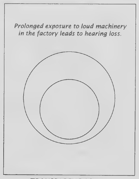Transparency 2-2-1: Hearing-loss argument

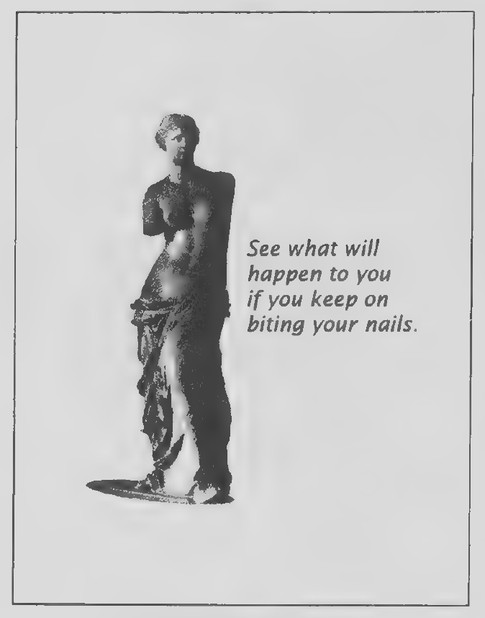Transparency 2-2-2: If you keep on biting your nails

Transparency 2-2-3: The squirrel problem

plane into three regions, two of which represent “not a” and two of which represent “not b.”

Lesson 2: Definitions

Lesson Outline

Terms: Definition, converse, if and only if.

Transparencies

• 2-2-1 Hearing-loss argument
• 2-2-2 If you keep on biting your nails
• 2-2-3 The squirrel problem

Review Rob Eastaway and Jeremy Wyndham relate the following legal case in their book titled Why Do Buses Come in Threes? The Hidden Mathematics of Everyday Life (Wiley, 1998):

“A man was suing his company for having caused his deafness. It was agreed by both sides that ‘prolonged exposure to loud machinery in the factory led to hearing loss.’… [T]he plaintiff’s argument was that this proved that his damaged hearing was due to prolonged exposure to loud machinery.”

Ask your students if they agree with this argument. Show Transparency 2-2-1. How would you change this sentence to “if-then” form? (If you are exposed to loud machinery in the factory for a long time, then this exposure leads to hearing loss.) What words belong in each circle of the Euler diagram? (“Loud machinery exposure” in the smaller circle and “hearing loss” in the larger circle.) If you have a hearing loss, does that mean that it was caused by exposure to loud factory machinery? This question leads naturally into a discussion of the converse of a

conditional statement, part of the new lesson. Alternative Review As a quick review, show Transparency 2-2-2 and ask, Of what kind of statement is “See what will happen to you if you keep on biting your nails” an example? (A conditional statement.) What is its hypothesis? (You keep on biting your nails.) What is the rest of the statement called? (The conclusion.) If an Euler diagram were drawn to represent the statement, which words would go in the smaller circle? (You keep on biting your nails.)

Introduction

The American philosopher William James told of camping with some friends in the mountains and returning from a walk to find them engaged in a heated argument. Scot Morris relates the story in his Next Book of Omni Games (New American Library, 1988): “It seems that one of the men had come upon a squirrel clinging to a tree trunk [Transparency 2-2-3]. As the man circled the tree, the squirrel did the same, so that it always faced the man. After going once around the tree, they were both back to where they started. It was clear that the man and the squirrel had both gone around the tree. The question was, Did the man go around the squirrel?” Before giving your students James’s answer, you might poll them about what they think. Morris summarizes it as follows: “If by around we mean ‘First to the south of, then to the west of, then to north of, then to east of…’ then the man does go around the squirrel. If around means ‘First in front of, then to the left of, then in back of, then to the right of.. then, of course, he doesn’t.”

This story leads into the rest of the new lesson.

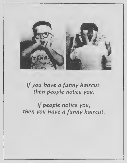Transparency 2-3-1: If you have a funny haircut

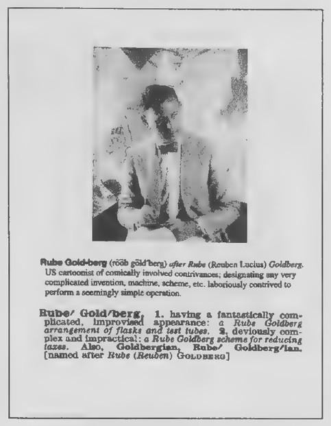Transparency 2-3-2: Rube Goldberg dictionary entry

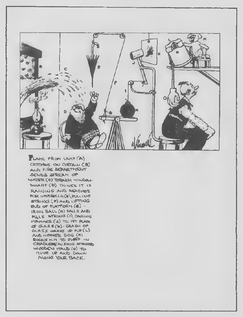Transparency 2-3-3

A convenient example to use that is different from the one in the text is the definition of “concurrent lines.” You might have your students write it in all three forms as you introduce the ideas of converse and iff:

If lines are concurrent, then they contain the same point.

If lines contain the same point, then they are concurrent.

Lines are concurrent if and only if they contain the same point.

Background for the Teacher In the chapter titled “The Role of Definitions” in his book titled Euclid—The Creation of Mathematics (Springer, 1999), Benno Artmann states: “After Blaise Pascal… it became firmly established that in mathematics definitions are what are called nominal definitions. The notion ‘square’ is nothing but an abbreviation of the phrase ‘equilateral and equiangular quadrilateral,’ and the same is true for any other mathematical concept. In principle one should always be able to replace the shorthand notion by the terms that were used in its definition. In fact, many routine proofs do just this. And more than that: Definitions are never right or wrong, but can only be more or less useful.”

Lesson 3: Direct Proof

Lesson Outline

Terms: Syllogism, direct proof (premises, conclusion), theorem.

Ideas: Pattern of direct proof.

Transparencies

• 2-3-1 If you have a funny haircut
• 2-3-2 Rube Goldberg dictionary entry
• 2-3-3 . Rube Goldberg cartoon
• 2-3-4 Aristotle and the syllogism
• 2-3-5 The yellow rows of taxis (Set I, Exs. 17 and 18)
• 2-3-6 Tick-tack-toe proofs (Set II, Exs. 29-32)

Review Show just the photograph at the upper left of Transparency 2-3-1 and then the photograph at the upper right. These pictures are of three-year-old Robert Eugene Powell of Wichita Falls, Texas, whose father cut his hair in the shape of a coonskin cap when Davy Crockett was popular in the early days of television. Compare the statements below the photographs: (1) If you have a funny haircut, then people notice you. (2) If people notice you, then you have a funny haircut. Do these statements say the same thing? (Observe that, although the first statement may be true, the second certainly is not.) In what way is the second statement related to the first? (It is the converse of the first.) There is one type of statement in mathematics for which the converse is always true. What kind of statement is it? (A definition.) Why is the converse of a definition always true? (The word being defined and its definition have the same meaning.)

Introduction

Show Transparency 2-3-2. Rube Goldberg was an American artist whose name now appears in many dictionaries owing to his drawings of crazy inventions. There are even Rube Goldberg contests the purpose of which is to build the most complicated

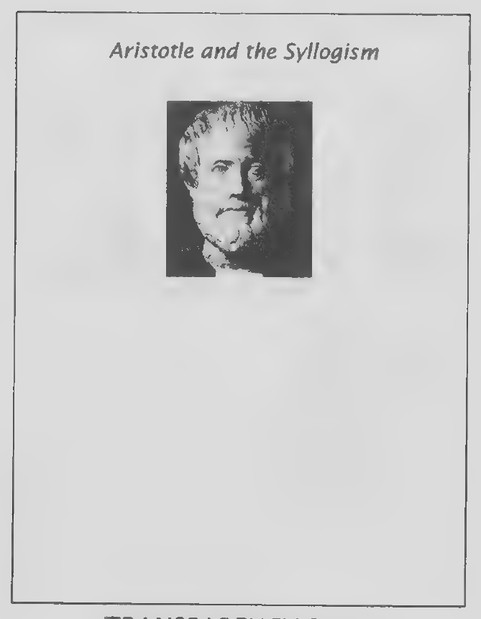Transparency 2-3-4: Aristotle and the syllogism

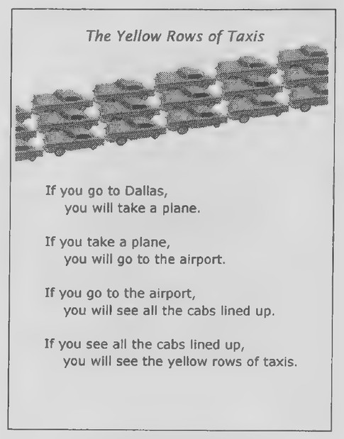Transparency 2-3-5: The yellow rows of taxis (Set I, Exs. 17 and 18)

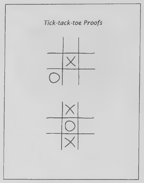Transparency 2-3-6: Tick-tack-toe proofs (Set II, Exs. 29-32)

Transparency 2-4-1: Sea lion solving logic problem

machine possible to perform a simple everyday task. (Your students might enjoy Rube Goldberg Inventions by Maynard Frank Wolfe (Simon & Schuster, 2000) as well as the Web site www.rube-goldberg.com.) The cartoon on Transparency 2-3-3 is for use in illustrating the idea of a direct proof as in the lesson in the text. Explain that the cartoon depicts an outlandish device for scratching a person’s back. If the curtain catches fire, the fire department will send water through the window; if water comes through the window, the man by the window will think it is raining—and so on—until, if the pup’s cradle is rocked, the wooden hand will scratch the man’s back. If all of the premises are true, we can conclude that, “if the curtain catches fire, then the wooden hand will scratch the man’s back.”

After representing the pattern of the argument in symbols, you can use Transparency 2-3-4 to illustrate the shortest such argument, the syllogism. The photograph is of a marble bust of Aristotle, the Greek philosopher and scientist who lived about a hundred years before Euclid. The work of Aristotle on the subject of logic is credited for contributing indirectly to Euclid’s Elements. It was in Aristotle’s writings that the syllogism was first discussed. The words “syllogism” and “logic” both derive from the Greek word “logos,” meaning “word” or “reason.”

Lesson 4: Indirect Proof

Lesson Outline

Terms: Indirect proof.

Ideas: Pattern of indirect proof.

Transparencies

• 2-4-1 Sea lion solving logic problem
• 2-4-2 . Anno’s Hat Tricks book cover
• 2-4-3 . Anno’s hat tricks
• 2-4-4 The third hat trick explained
• 2-4-5 Trading desks proof (Set II, Ex. 15)
• 2-4-6 Poker proof (Set II, Ex. 17)
• 2-4-7 Balanced weights puzzles (Set II, Ex. 18)

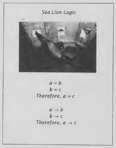
Review Scientific researchers working with sea lions have found that these animals can solve simple problems in logic. The photograph on Transparency 2-4-1 shows a seal comparing three different symbols. If the seal has learned that symbols a and b are equivalent and that symbols b and c are equivalent, it concludes that symbols a and c are equivalent.

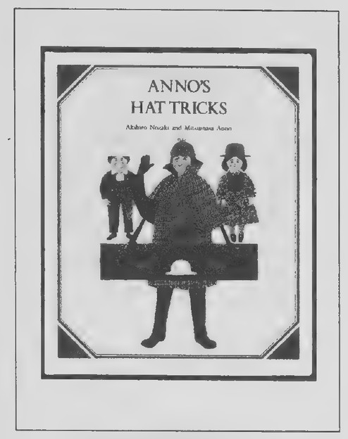Transparency 2-4-2: HAT TRICKS

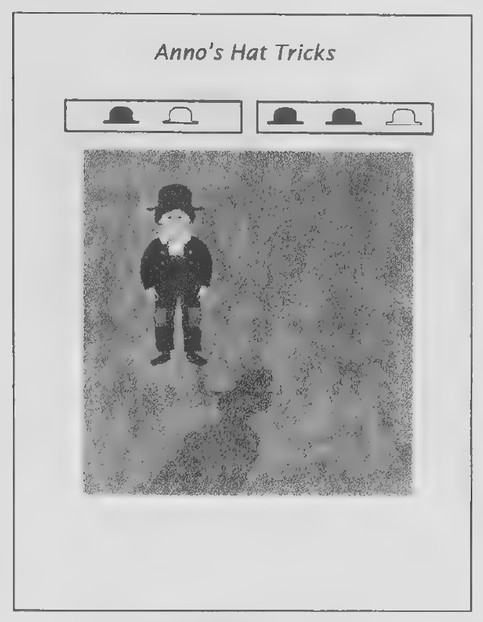Transparency 2-4-3: Anno’s Hat Tricks

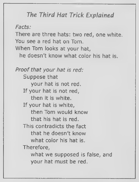Transparency 2-4-4: The third hat trick explained

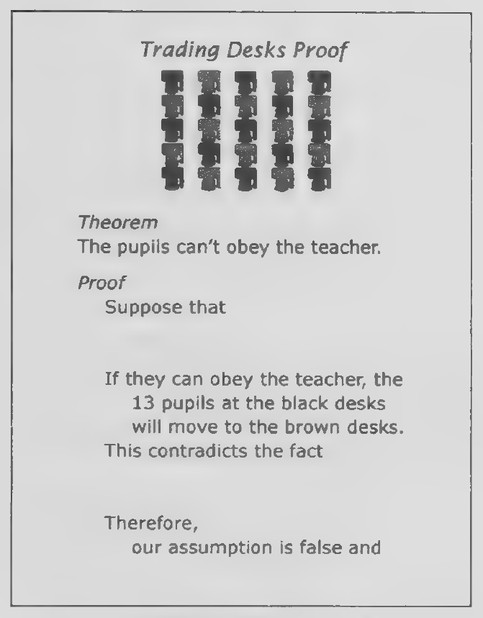Transparency 2-4-5: Trading desks proof (Set II, Ex. 15)

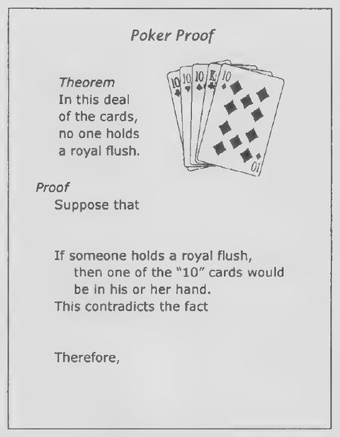Transparency 2-4-6: Poker proof (Set II, Ex. 17)

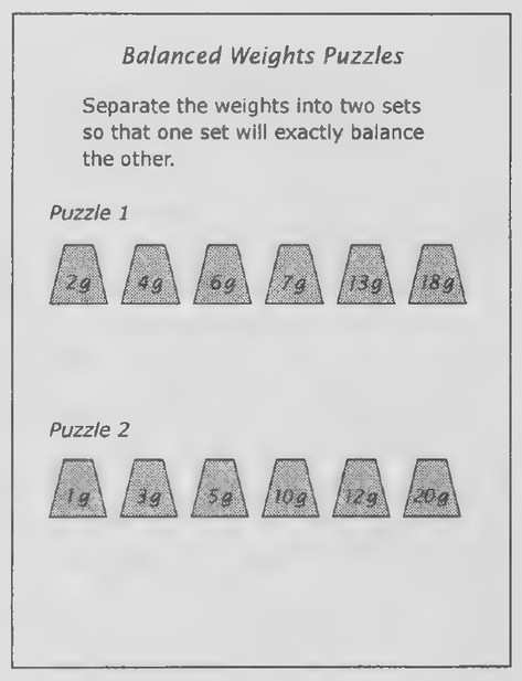Transparency 2-4-7: Balanced weights puzzles (Set II, Ex. 18)

Compare the two arguments below the photograph: a = b, b =c, therefore, a=c;anda—>b,b-—c, therefore, a — c. The first of these arguments is of the type with which you became acquainted in algebra: in it, a, b, and c represent numbers, and the three statements are equations. The second argument is of the type with which you have become acquainted in geometry. What do a, b, and c represent in it? (Phrases.) What are the three individual statements called? (Conditional statements.) What is the pattern of the three statements called? (A syllogism.) What kind of proof does a syllogism demonstrate? (A direct proof.) The first two statements are the premises of the argument. What is the third statement called? (The conclusion.) What is a statement that is proved by reasoning deductively from

already accepted statements called? (A theorem.)

Introduction

The book Anno’s Hat Tricks with text by Akihiro Nozaki and pictures by Mitsumasa Anno (Transparency 2-4-2) includes a series of entertaining puzzles that provide a good introduction to indirect proof. The following list outlines how the puzzles develop:

1. A hatter has one red hat and one white

hat. He puts a hat on Tom and a hat on

you. Tom looks at your hat and concludes

that his own hat is red. What color is your

hat? (White.)

2. The hatter takes two red hats and one

white hat. He puts a hat on Tom and a hat

on you. You see that Tom’s hat is red. Tom

looks at your hat and concludes that his

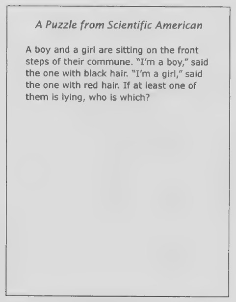Transparency 2-5-1: A puzzle from Scientific American

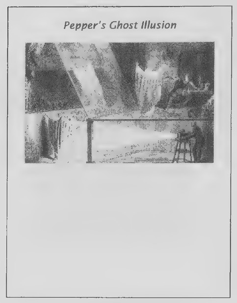Transparency 2-5-2: Pepper’s ghost illusion

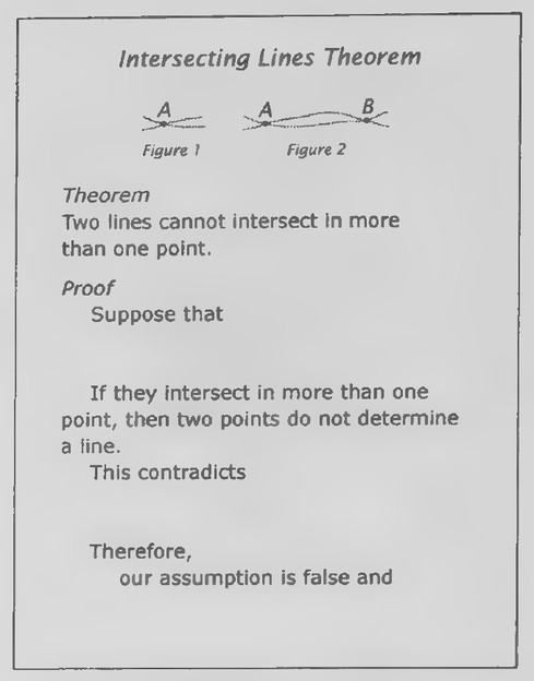Transparency 2-5-3: Intersecting lines theorem (Set II, Ex. 41)

own hat is red. What color is your hat?

(White. Otherwise, Tom wouldn’t have

known that his hat was red.)

3. The hatter again takes two red hats and

one white hat. He puts a hat on Tom and

ahat on you. You see that Tom’s hat is red.

Tom looks at your hat but doesn’t know

what color his hat is. What color is your

hat? (Red. Otherwise, Tom would know

that his hat was red.) Although these tricks are considered in the text, your class might enjoy seeing these puzzles enacted with two students: one playing Tom and facing the class; the other playing you (the reader of the book) and facing Tom. Alternatively, you might show Transparency 2-4-3 with the upper right box showing three hats covered. After the first puzzle, cover the upper left box, uncover the upper right box and proceed with the remaining puzzles. Transparency 2-4-4 contains the final argument put into the format of an indirect proof as in the text. The most effective way to use it is to begin with the transparency covered with a sheet of paper and then slide the paper downward to enable your students to anticipate the progression of the proof.

Lesson 5: A Deductive System

Lesson Outline

Terms: Undefined terms, postulate, theorem, deductive system.

Postulate 1: Two points determine a line.

Postulate 2: Three noncollinear points determine a

plane.

Transparencies

• 2-5-1 A puzzle from Scientific American
• 2-5-2 Pepper’s ghost illusion
• 2-5-3 Intersecting lines theorem (Set II, Ex. 41)
• 2-5-4 How many lines? (Set III)

Review The puzzle on Transparency 2-5-1 once appeared in Martin Gardner’s “Mathematical Games” column in Scientific American July 1971) and provides a good review of indirect reasoning:

“A boy and a girl are sitting on the front steps of their commune. ‘I’m a boy,’ said the one with black hair. ‘I’m a girl,’ said the one with red hair. If at least one of them is lying, who is which?”

As Gardner explains, there are four possible true-false combinations for the two statements: TT, TE FT, and FF. The first is eliminated because it contradicts the fact that at least one of the two is lying. The second and third are eliminated because they lead to the conclusions that both are boys or both are girls, each of which contradicts the fact that one is a boy and one is a girl. So we are left with the conclusion that both lied. The person with black hair is a girl and the person with red hair is a boy.

Introduction

A very popular entertainment in London in 1862 was Pepper’s Ghost Illusion. Something similar to it is used in the Haunted House in Disneyland. The picture on Transparency 2-5-2 shows how the ghost illusion worked. A large sheet of glass was set up on a stage so that it was tilted toward the audience. An actor playing a ghost stood below the level of

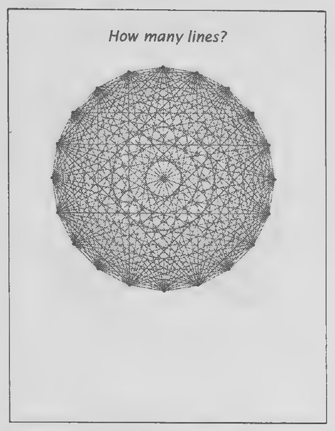Transparency 2-5-4: How many lines? (Set III)

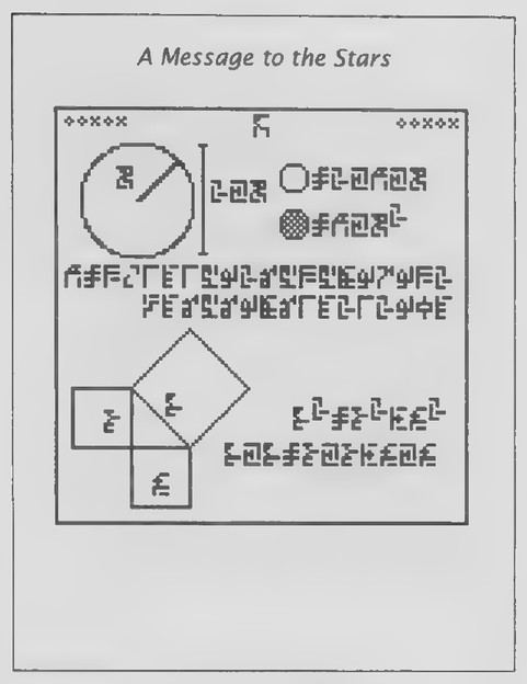Transparency 2-6-1: A message to the stars

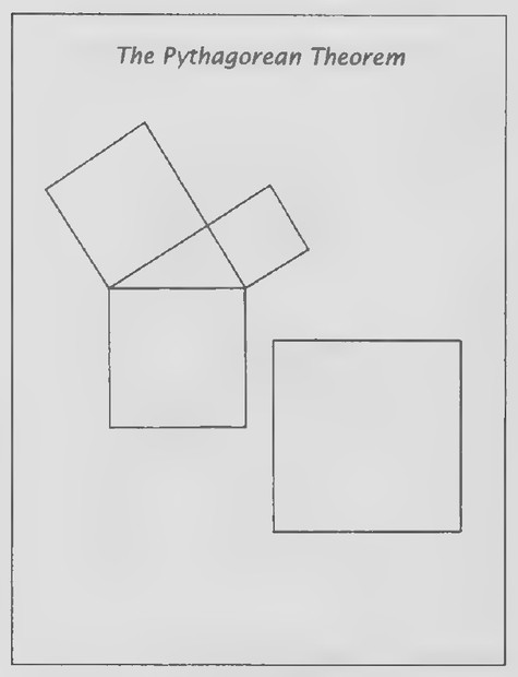Transparency 2-6-2: The Pythagorean Theorem

the stage. Light projected onto the actor was reflected onto the glass, creating the illusion of a ghost interacting with the actors on the stage. The lighting in the theater was such that the audience saw the ghost but not the glass, and the resulting effect caused a sensation.*

This illusion was based on clever lighting and some three-dimensional geometry. To understand how it works, it is convenient to think of the positions of the real ghost and the illusion on the stage as points, the light producing the illusion as traveling along lines, and the plate of glass and the floor of the stage as parts of planes.

After this introduction, the rest of the lesson can be presented as in the text. Having your students make the following outline should help them understand the components of a deductive system.

A Deductive System

Undefined terms: to avoid circularity.

Definitions.

Postulates (assumed statements): to avoid cir-

cularity.

Theorems (proved statements): proved directly

or indirectly by using rules of logic.

Lesson 6: Some Famous Theorems of Geometry

Lesson Outline

Terms: Hypotenuse, circumference, diameter, pi.

The Pythagorean Theorem: The square of the hypotenuse of a right triangle is equal to the sum of

the squares of the other two sides. The Triangle Angle Sum Theorem: The sum of the

angles of a triangle is 180°. Two Circle Theorems: If the diameter of a circle is d,

its circumference is πd. If the radius of a circle

is r, its area is πr.

Transparencies

• 2-6-1 A message to the stars
• 2-6-2 The Pythagorean Theorem
• 2-6-3 The Triangle Angle Sum Theorem

Introduction

In 1999, two Canadians, astrophysicist Yvan Dutil and cryptographer Stephane Dumas, sent a message into space in the hope of reaching extraterrestrial intelligence. Called the Evpatoria Message or Cosmic Call, it consisted of 23 pages of information about our mathematics, ourselves, Earth, and our solar system.’ Page 5 is about geometry and is reproduced on Transparency 2-6-1. I suggest making copies of this page so that your students can mark it as you consider it in class. The figures and the symbols accompanying them represent three of the most useful and famous theorems of geometry. Can you guess what either figure is about? (The first figure shows a circle with a radius. The symbol by the radius represents its length, R, and the vertical segment to the right of the circle represents the length of its diameter. To the immediate right of this segment are three symbols representing 2 x R. The two rows of symbols to the right of these symbols

*The Great Illusionists, by Edwin A. Dawes (Chartwell Books, 1979).

tThe entire message can be found on the Web site www3.sympatico.ca/stephane_dumas/CETI/ #1999_MESSAGE.

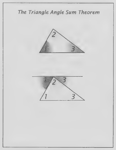Transparency 2-6-3: The Triangle Angle Sum Theorem

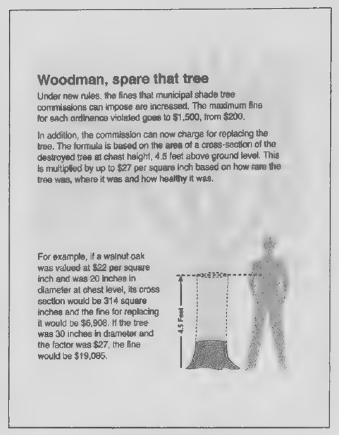Transparency 2-R-1: Woodman, spare that tree

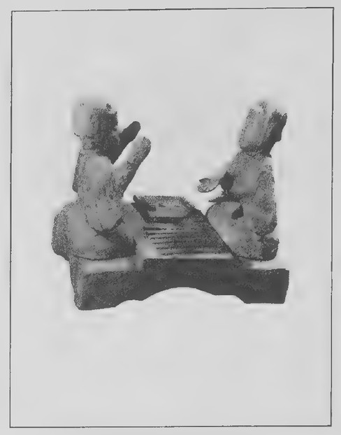Transparency 2-R-2: Backgammon sculpture

represent C = 2x mx Rand A= R². The two long rows of symbols directly below list some of the digits of 1. (m7 = 3.14159…)

The lower figure, showing squares drawn on the three sides of a right triangle, represents the Pythagorean Theorem. The three symbols on the sides, starting with the hypotenuse and reading clockwise, are c, b, and a. The two rows of symbols to the right of the figure represent c² = a² + b² and cXc=axat+bxb.

Although formal proofs of the theorems of Lesson 6 will not be considered until later in the course, you will want to present the area demonstration of the Pythagorean Theorem illustrated at the top of page 66 of the text. Transparency 2-6-2 can be used for this purpose. In advance of class, cut from thick sheets of colored plastic the three squares and four copies of the triangle shown in the top figure of the transparency. The triangles should be one color and the squares another. Place the three squares and one of the triangles on the transparency figure and point out that we want to show that it is reasonable to think that the sum of the areas of the two smaller squares is equal to the area of the largest one. Then arrange the triangle and large square in the frame at the bottom of the transparency as shown in the third figure at the top of page 66 of the text. Fill in the remaining spaces with the other three triangles. Explain that we can remove the large square and rearrange the four triangles so that there is exactly enough room for the two smaller squares. In this demonstration, you might leave the triangle at the lower left in place and slide the other three triangles to the appropriate positions so that the two smaller

squares can be fitted into place.

Transparency 2-6-3 is for use in illustrating the Triangle Angle Sum Theorem.

Review of Chapter 2

Transparencies

• 2-R-1 _ Woodman, spare that tree
• 2-R-2 Backgammon sculpture
• 2-R-3 Some rules of backgammon
• 2-R-4 Putting knowledge to work
• 2-R-5 Dialogue with an expert system
• 2-R-6 Expert system’s explanation

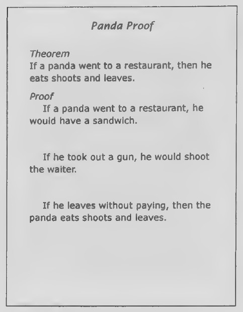
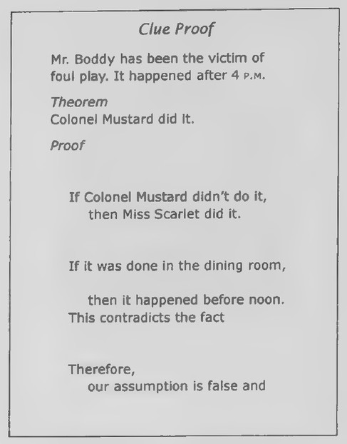
2-R-7_ Panda proof (Set II, Exs. 40 and 41) 2-R-8 Clue proof (Set II, Exs. 42 and 43) 2-R-9 Circle in the square (Set II, Exs. 4449)

First day

Introduction

A newspaper article tells of rules establishing fines for cutting down city shade trees. According to the article, “The formula is based on the area of a crosssection of the destroyed tree at chest height, 4.5 feet above ground level. This is multiplied by up to $27 per square inch based on how rare the tree was, where it was and how healthy it was.”

Checking the numbers in the example in the article provide a good exercise for your students in reviewing the formula for the area of a circle. The example is somewhat strange for two reasons. First, a tree with a 20-inch diameter has a radius of 10 inches. The cross-sectional area of 314 square inches clearly comes from letting 7 = 3.14. Students using the m key on a calculator will get an area of 314.159… Square inches and a fine of $6,911.50 rather than

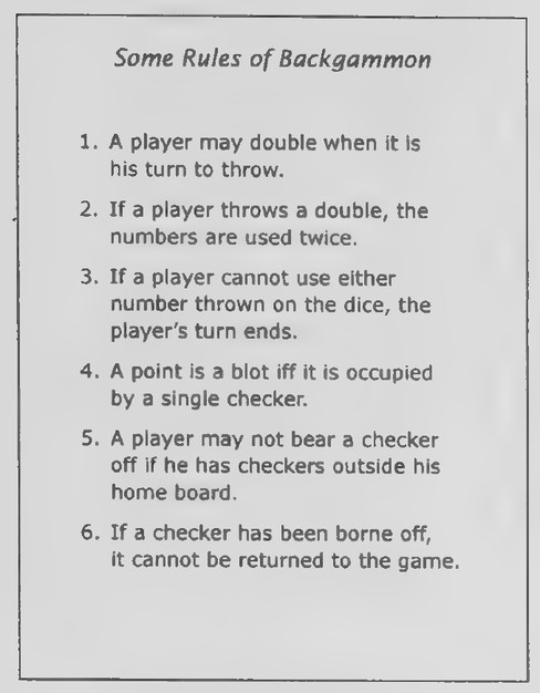Transparency 2-R-3: Some rules of backgammon

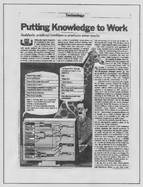Transparency 2-R-4: Putting knowledge to work

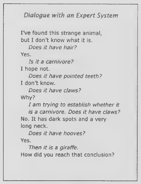Transparency 2-R-5: Dialogue with an expert system

$6,908. Second, if we continue to letnm =3.14, thena tree with a 30-inch diameter has a cross-sectional area of (3.14)(15)* = 706.5 square inches; a fine factor of $27 gives $19,075.50, rather than $19,085. On the other hand, if the mt key on the calculator is used, the fine becomes about $19,085, the number reported in the article!

Second day

Introduction

Show Transparency 2-R-2 and ask if anyone can guess what game the two people in the picture are playing. (It looks like backgammon.) Amazingly, the photograph is of a sculpture found by Chinese archeologists in a second-century tomb. Some of the rules of backgammon are listed on Transparency 2-R-3:

1. A player may double when it is his turn to

throw. 2. If a player throws a double, the numbers are

used twice. 3. If a player cannot use either number thrown

on the dice, the player’s turn ends. 4. A point is a blot iff it is occupied by a single

checker. 5. A player may not bear a checker off if he has

checkers outside his home board. 6. If a checker has been borne off, it cannot be

returned to the game.

What kind of statements are these rules? (Conditional statements.) What is the hypothesis of statement 1? (When it is his turn to throw.) What is the conclusion of statement 3? (The player’s turn ends.) Which statement is a definition? (Statement 4.) What

does the symbol “iff” in this statement mean? (If and only if.) Is the converse of every definition true? (Yes.) Why? (Because the word being defined and its definition have the same meaning.) In general, if a conditional statement is true, is it correct to conclude that its converse is true? (No.) Most rules of games are assumed to be true without proof. What are such statements called in geometry? (Postulates.) What do we call statements that are proved? (Theorems.)

Alternate Introduction An important branch of computer science is artificial intelligence or AI. Artificial intelligence has been defined as “the study of the computations that make it possible to perceive, reason, and act.” Its goal is to understand and emulate the ability of humans to reason; included in every AI program are the rules of deductive reasoning. AI programs called expert systems are now used in a wide variety of applications ranging from business to engineering to medical care. An example of a simple expert system illustrated on Transparency 2-R-4 shows how a series of questions lead to the identification of an animal. The dialogue is reproduced on Transparency 2-R-5:

I’ve found this strange animal, but I don’t

know what it is.

Does it have hair?

Yes.

Is it a carnivore?

I hope not.

Does it have pointed teeth?

I don’t know.

Transparency 2-R-6: Expert system’s explanation

Transparency 2-R-7: Panda Proof

Transparency 2-R-8: Clue proof (Set II, Exs. 42 and 43)

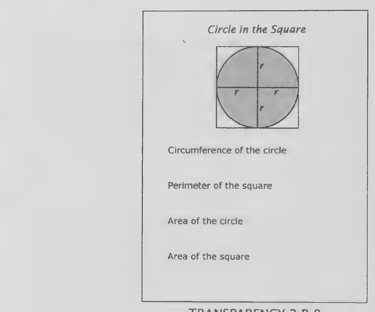Figure on page 308 — A worksheet table of circle and polygon measurements (circumference, perimeter, area)

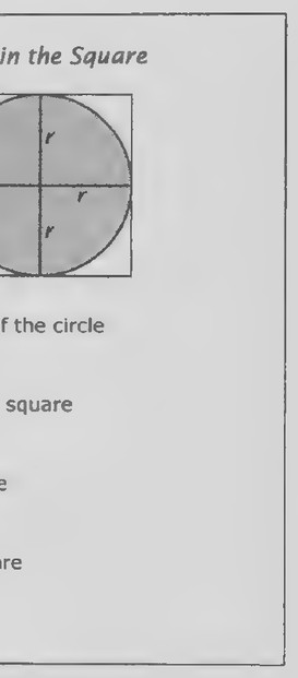Transparency 2-R-9: Circle in the square (Set II, Exs. 4449)

Does it have claws?

Why?

Iam trying to establish whether it is a carnivore.

Does it have claws?

No. It has dark spots and a very long neck.

Does it have hooves?

Yes.

Then tt is a giraffe.

° A

How did you reach that conclusion?

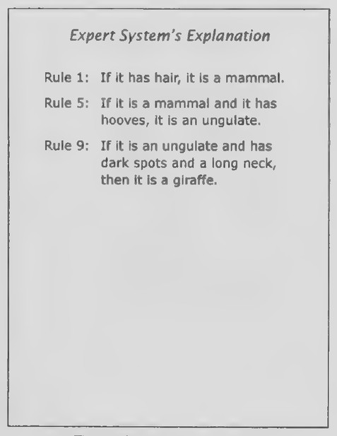
The expert system’s answer is reproduced on Transparency 2-R-6:

Rule 1: If it has hair, it is a mammal.

Rule 5: If it is a mammal and it has hooves, it is an

ungulate.

Rule 9: If tt ts an ungulate and has dark spots and

a long neck, then it is a giraffe.

These rules can be used to provide a brief review of conditional statements. They also provide an example of a chain of statements similar to but somewhat more complicated than a > b, b> c, c — d. The flow chart at the bottom of the figure on Transparency 2-R-4 is comparable to the structure of a complex proof in geometry.

Circle

of the

circle

square TRANSPARENCY

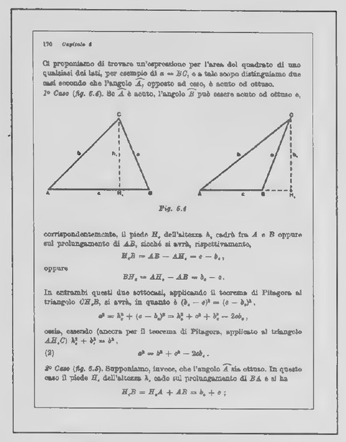Transparency 3-1-1: Page from Italian geometry book

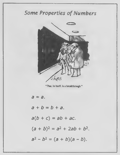Transparency 3-1-2: Some properties of numbers

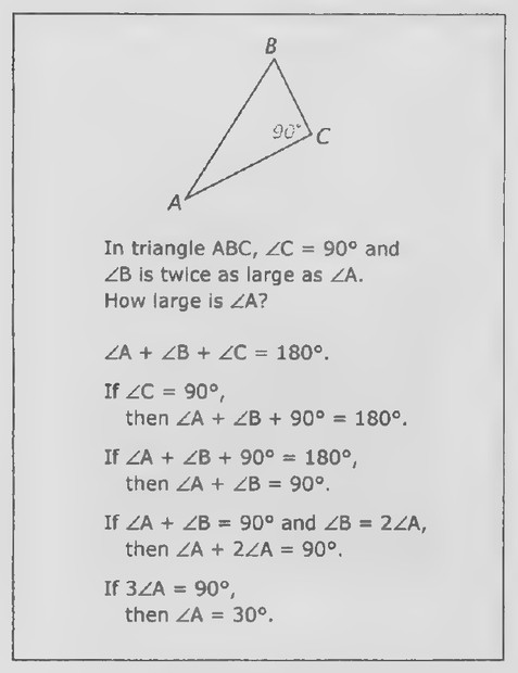Transparency 3-1-3: Properties of equality applied to a geometric figure

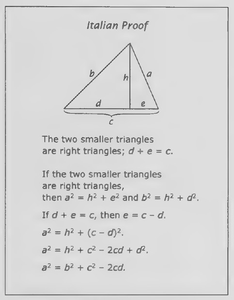Transparency 3-1-4: Italian proof

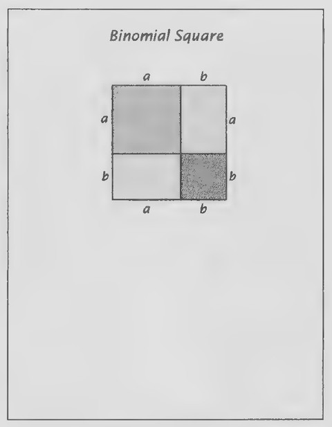Transparency 3-1-5: Binomial square (Set II, Exs. 25-30)

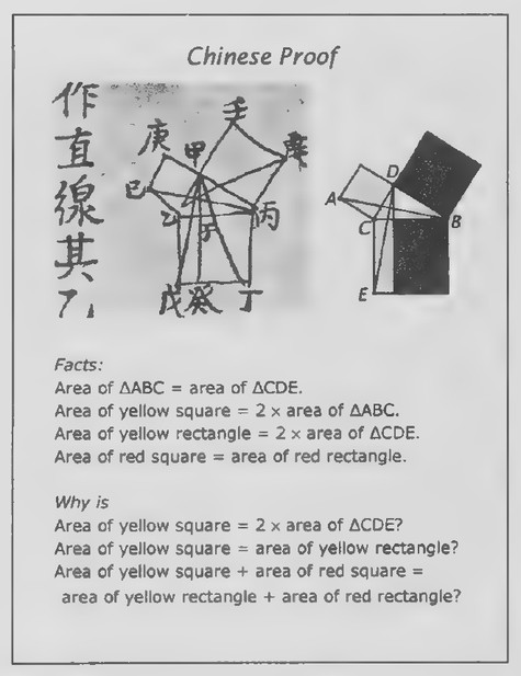Transparency 3-1-6: Chinese proof (Set II, Exs. 31-35)

Chapter 3: Lines and Angles

Lesson 1: Number Operations and Equality

Lesson Outline

Terms: Axiom, equal.

Properties of equality: Reflexive, substitution, addition, subtraction, multiplication, division.

Transparencies

• 3-1-1 Page from Italian geometry book
• 3-1-2 Some properties of numbers
• 3-1-3 Properties of equality applied to a geometric figure
• 3-1-4 Italian proof
• 3-1-5 Binomial square (Set II, Exs. 25-30)
• 3-1-6 Chinese proof (Set II, Exs. 31-35)

Introduction

The lessons in Chapter 2 ended with one on some famous theorems of geometry. Each of these theorems included information that can be stated in the form of an equation: c² = a² + b², ∠1 + ∠2 + ∠3 = 180°, C = πd, A = πr². The page from the Italian geometry book reproduced on Transparency 3-1-1 illustrates the fact that equations are also used in writ-

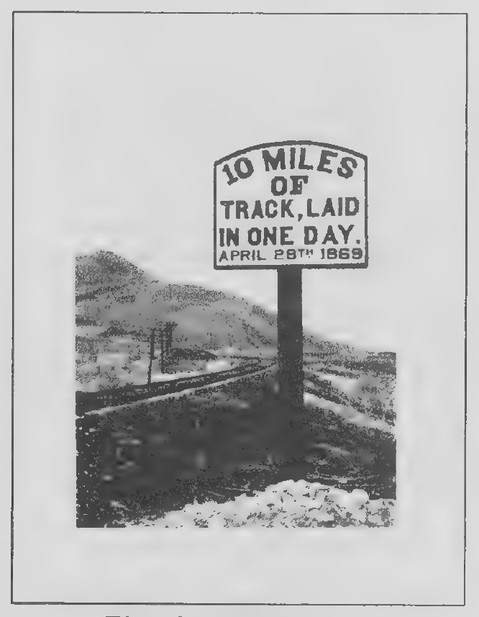Transparency 3-2-1: Transcontinental railroad sign

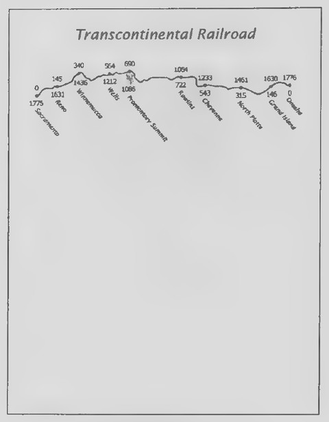Transparency 3-2-2: Transcontinental railroad map

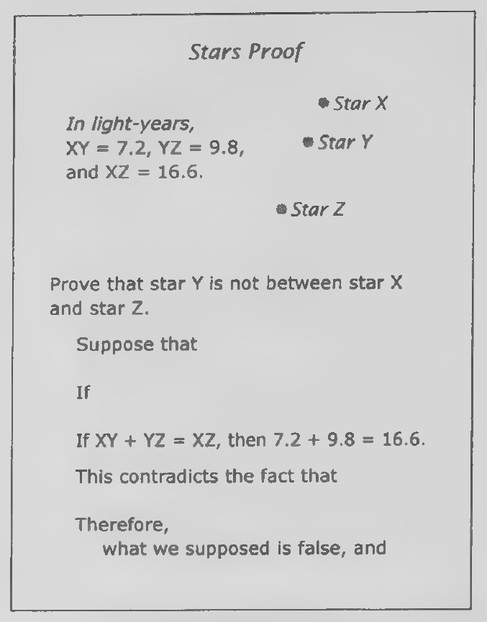Transparency 3-2-3: Stars proof (Set II, Ex. 45)

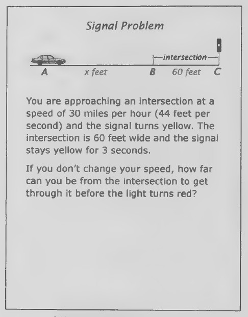Transparency 3-2-4: Signal problem (Set II, Ex. 46)

ing geometric proofs. (Observe also that there are two references to “il teorema di Pitagora” on this page.) In this lesson, we consider some of the properties of numbers and equations and add them to our logical system. Transparencies 3-1-2 and 3-1-3 are for possible use in developing the lesson as in the text. In using Transparency 3-1-3, keep the statements beginning with ∠A + ∠B + ∠C = 180° covered until your students have had a chance to try to figure out the measure of ∠A. Then reveal the lines of the proof one at a time so that your students can anticipate the steps, as well as giving the reasons. If your students are up to it, you might have them take a further look at some of the proof on the page from the Italian geometry book. (Although it is a development of the Law of Cosines, I suggest that you not mention this fact to your students at this point.) Transparency 3-1-4 can be used for this purpose. Again, uncover the steps as your students consider how they are explained.

Lesson 2: The Ruler and Distance

Lesson Outline

Terms: Ruler, coordinate, distance, between (points).

Postulate 3. The Ruler Postulate: The points on a line can be numbered so that positive number differences measure distances.

Definition: Betweenness of points.

Theorem 1. The Betweenness of Points Theorem. If A-B-C, then AB + BC = AC.

Transparencies

• 3-2-1 Transcontinental railroad sign
• 3-2-2 Transcontinental railroad map
• 3-2-3 Stars proof (Set II, Ex. 45)
• 3-2-4 Signal problem (Set II, Ex. 46)

Introduction

Show Transparency 3-2-1. Although the date on this sign is April 28, 1869, it was an event 2 weeks later that became famous in American history. Do you know what the event was? (The transcontinental railroad was completed on May 10.) Before the completion of this railroad, it took at least 4 months to travel across the United States. Afterward, the trip could be made in just 1 week.

Hand out duplicated copies of Transparency 3-2-2 to your students. Before 1865, railroad tracks had been built from the east coast as far west as Omaha,

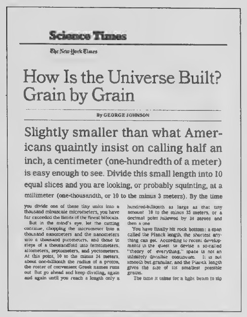Transparency 3-3-1: How is the universe built?

Transparency 3-3-2: Smaller and smaller

Transparency 3-3-3: Points of sailing

Nebraska. In that year, Union Pacific began laying tracks westward at the same time that Central Pacific was laying tracks eastward from Sacramento. It was Central Pacific that managed to put down 10 miles of tracks in just 1 day just before the two tracks met at Promontory Summit just north of the Great Salt Lake. Two sets of numbers appear on the map on Transparency 3-2-2. What do you suppose they represent? (The distances in miles of the indicated points along the railroad from Sacramento and from Omaha.) How many miles of track did Central Pacific lay from Sacramento to Promontory Summit? (690.) How many miles of track did Union Pacific lay from Omaha to Promontory Summit? (1,086.) How many miles of track connected Reno to Cheyenne? (1,088.) Explain that the two sets of numbers are two coordinate systems. The question about the distance from Reno to Cheyenne reveals that the distance between two points can be found as the positive difference between their coordinates. Further examples from the railroad map can be used to develop the rest of the lesson, including the Ruler Postulate and the ideas concerning betweenness of points. Some students may enjoy learning more about the construction of the transcontinental railroad from the Web site, www.pbs.org/wgbh/ amex/tcrr/sfeature/sf_map.html, which also features an attractive interactive map.

Lesson 3: The Protractor and Angle Measure

Lesson Outline

Terms: Protractor, degree, rotation of rays, half-

rotation of rays, coordinate, measure of angle,

acute, right, obtuse, straight, between (rays). Postulate 4. The Protractor Postulate: The rays ina

half-rotation can be numbered from 0 to 180

so that number differences measure angles. Definition: Betweenness of rays. Theorem 2: The Betweenness of Rays Theorem.

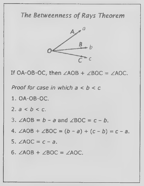
If OA-OB-OC, then ∠AOB + ∠BOC = ∠AOC.

Transparencies

• 3-3-1 How is the universe built?
• 3-3-2 Smaller and smaller
• 3-3-3 Points of sailing
• 3-3-4 Betweenness of Rays Theorem (Set II, Ex. 54)

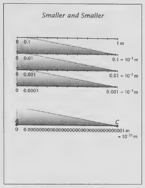
Review On Transparency 3-3-1 is the beginning of an article from the New York Times (December 7, 1999), about the structure of the universe. It concerns a property of physical space that seems almost impossible to believe because it is so contrary to our intuition. The Ruler Postulate is based on thinking of a ruler as an infinite number line. The points on the line are numbered so that to every point there corresponds exactly one real number called its coordinate and to every real number there corresponds exactly one point. Show Transparency 3-3-2. The figure at the top illustrates the division of a length of 1 meter into 10 equal parts called decimeters (idm=01 m= 10-1 m. The second figure shows the division of 1 decimeter into 10 equal centimeters (1 cm = 0.01 m = 10 m). The third figure shows 1 centimeter divided into 10 equal millimeters, the smallest length that you see marked on a ruler (1 mm = 0.001 m = 10° m). If we imagine continuing this process, we even-

Transparency 3-3-4: Betweenness of Rays Theorem (Set II, Ex. 54)

Transparency 3-4-1: Cat and rabbit vision

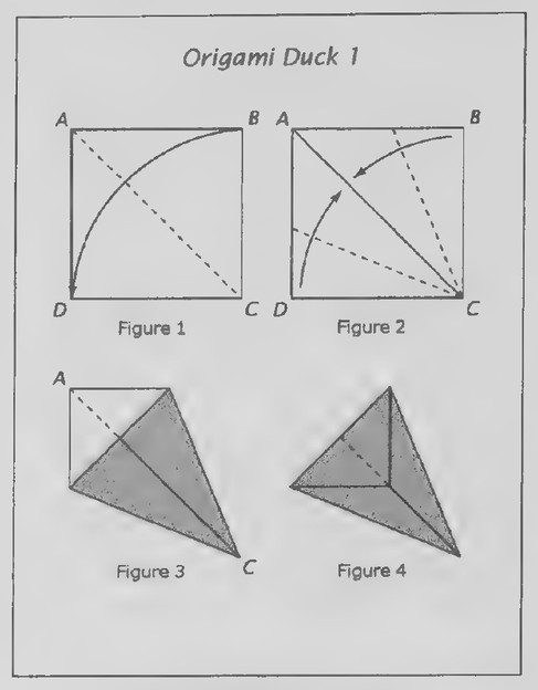Transparency 3-4-2: Origami duck 1

tually get to a length of 10-* m, and here is the surprise. As the Times article puts it: “You have finally reached rock bottom: a span called the Planck length, the shortest anything can get. According to recent developments in the quest to devise a socalled ‘theory of everything,’ space is not an infinitely indivisible continuum. It is not smooth but granular, and the Planck length gives the size of its smallest possible grains.”

It seems natural to be able to choose points between the points A and C that mark the endpoints of the Planck length. Just choose any number less than 10° and let it be the coordinate of the point. By our definition of betweenness of points, if the coordinate of the point, B, is n and 0 <n < 10°35, then A-B-C. The Ruler Postulate treats geometric “lines” as being “continuous,” meaning that they can be subdivided indefinitely. Physical “lines,” on the other hand, do not seem to be continuous in that they cannot be subdivided indefinitely! As J. L. Heilbron remarks in his Geometry Civilized (Clarendon Press, 1998): “None of these things—points, lines, or planes—exist in the word of immediate experience. And yet they exist. By the powerful act of your imagination, you have been able to conceive them clearly and distinctly.” This is a good reminder that, although geometry provides a powerful model of the physical world, the two are not the same.

Introduction

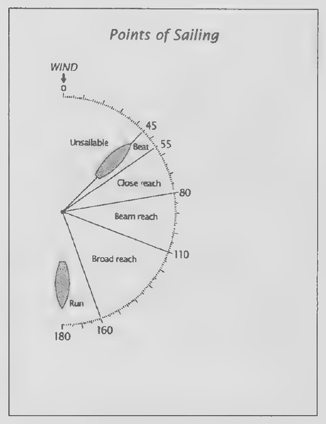
Hand out duplicated copies of Transparency 3-3-3. The protractor diagram shows some of the “points” of sailing. The arrow at the top indicates the direction of the wind. Most sailboats cannot sail nearer

than 45° toward the wind. A boat sailing at angle between 45° and 55° is said to be “beating” the wind. The protractor also shows the directions included in “close reaching,” “beam reaching,” “broad reaching,” and “running” with the wind. The diagram can be used to develop the lesson as in the text. You will probably not have time to make more than a brief outline of the statements of the definitions and theorem.

Lesson 4: Bisection

Lesson Outline

Terms: Bisect, midpoint, angle bisector, congruent, corollary.

Corollary to the Ruler Postulate: A line segment has exactly one midpoint.

Corollary to the Protractor Postulate: An angle has exactly one ray that bisects it.

Transparencies

• 3-4-1 Cat and rabbit vision
• 3-4-2 Origami duck 1
• 3-4-3 . Origami duck 2
• 3-4-4 Passion flower (Set II, Exs. 41-47)

Introduction

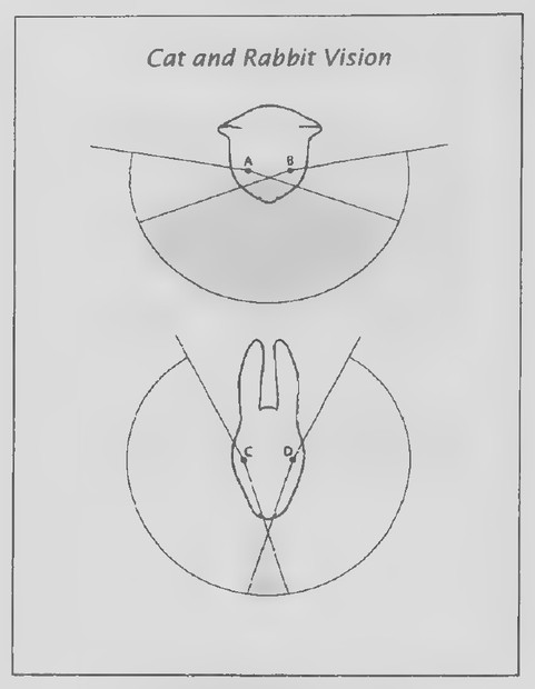
Hand out duplicated copies of Transparency 3-4-1. Cats and rabbits do not see the world in the same way. The eyes of a cat are positioned toward the front of its head. This positioning causes the visual fields of the eyes to overlap, and so the animal has good binocular vision (that is, it is able to see in three-dimensions). The eyes of a rabbit, on the other hand, are on either side of its head. As a result, the

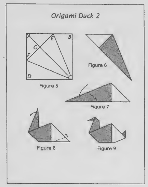Transparency 3-4-3

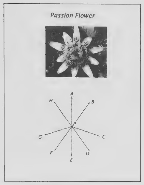Transparency 3-4-4: Passion flower (Set II, Exs. 41-47)

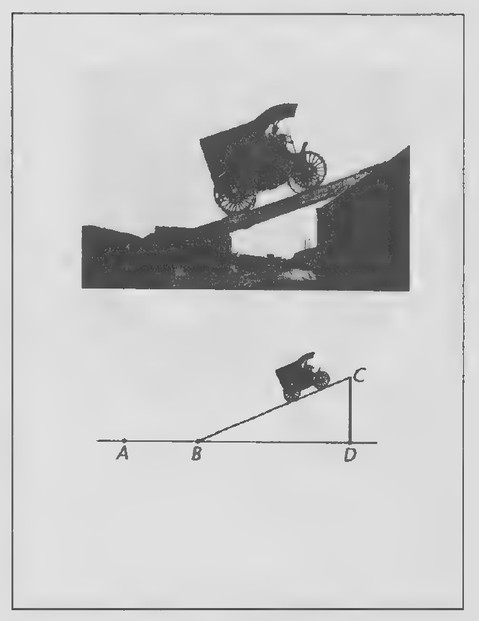Transparency 3-5-1: Popular Mechanics stunt

visual fields of the eyes have relatively little overlap, and so the rabbit has a much more panoramic view of its surroundings. In general, predatory animals have better binocular vision, whereas nonpredatory animals have better panoramic vision. To which animal is your vision more comparable? (The cat.) How does the vision of a horse compare with your vision? (It is flatter but more panoramic.)

How do the angles of the visual fields of the individual eyes of a cat and rabbit compare? Have your students use their protractors to measure the angles. (They are the same, about 170°.) To find the centers of the visual fields of the eyes, we can bisect these angles. Use your protractor to do so. We could also have bisected the angles by using a straightedge and compass. Suppose you had neither these tools nor a protractor. Can you think of another way that you might accurately bisect the angles? (By folding the paper.) The rest of the lesson can now be developed as in the text. Alternate introduction Because the lesson on bisection is developed around paper folding, your students might enjoy being introduced to it by folding the origami duck pictured on page 101 of the text. I suggest using squares of paper measuring about 5 inches on a side. Illustrations for doing the folding are shown on Transparencies 3-4-2 and 3-4-3, and the directions, all from Peter Engel’s Folding the Universe (Vintage Books, 1989), are given below:

1. Fold corner B over onto corner D. Unfold the

paper flat again (Figure 1).

2. Fold sides BC and DC onto the fold AC (Fig-

ures 2 and 3).

3. Fold corner A over onto the line where sides

BC and DC meet as shown by Figure 4.

4. Unfold the paper flat again and label the

points indicated on Figure 5.

Before proceeding any further, ask the following questions. Which angles were bisected by the first fold? (The angles at A and C.) Which angles were bisected next? (∠DCA and ∠BCA.) Can you find any more angles that have been bisected? (∠FCE and the straight angles at G. We know that ∠FCE has been bisected because ∠DCA = ∠BCA

and so = DCA = + 2BCA; ∠EeA= = DCA and

1 ∠ECA = a oBCA; so ∠FCA = ∠ECA by substitu-

tion.) Can you find any line segments that have been bisected? (FE.) Introduce the word congruent in this discussion.

The remaining steps are a bit more complicated:

5. Fold the paper so that it looks like figure 3

again.

6. Refold along AC so that label A appears on

the outside rather than the inside (Figure 6).

7. Turn the figure so that it is in the position

shown in Figure 7.

8. Fold the lower left part inward as shown in

Figure 8 to form the neck.

9, Fold the top of the neck inward to form the

head and the lower right part inward to form

the tail (Figure 9).

The rest of the lesson can now be presented as in the text.

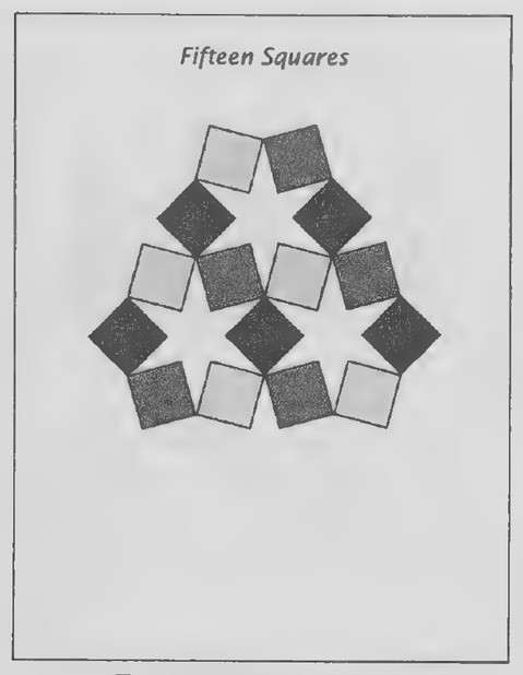Transparency 3-5-2: Fifteen squares (Set III)

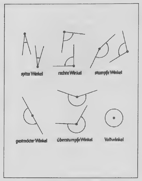Transparency 3-6-1: German angles

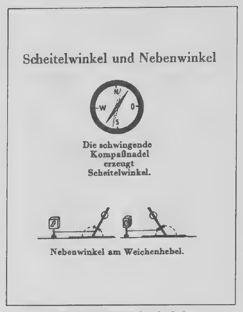Transparency 3-6-2: German angle relations

Lesson 5: Complementary and Supplementary Angles

Lesson Outline

Terms: Complementary (complement), supplementary (supplement).

Theorem 3. Complements of the same angle are equal.

Theorem 4. Supplements of the same angle are equal.

Transparencies

• 3-5-1 Popular Mechanics stunt
• 3-5-2 Fifteen squares (Set III)

Introduction

In the early days of automobiles, motorists frequently had to get out of their cars and push them when they came to a slight grade. The photograph on Transparency 3-5-1 is from a 1902 issue of Popular Mechanics magazine and shows a car being driven up a ramp to the top of a house. The purpose of the photograph was to demonstrate the power and grade-climbing ability of the car, both of which were unusual for the time. Modern cars are more powerful but also a lot heavier. It is hard to imagine such a stunt being carried out today!

The drawing below the photograph represents the ramp, the side of the house, and the ground. Guide your students in making a copy of it by doing the following:

1. Draw a horizontal line to represent the

ground. Mark a point B on it to represent

the bottom of the ramp and a point D to

represent the base of the house.

2. Use your protractor to draw a line to

represent the ramp, given that it rises 23°

with the ground.

3. Use the protractor to draw a line at D to

represent the side of the house.

4. Label the point C in which these two lines

intersect to represent the top of the ramp.

5. Choose and label a point A on the ground

line as shown in the figure.

Ask your students to measure ∠C, the angle that the ramp makes with the side of the house. Can you think of a way to figure out the size of ∠C without measuring it? (By the Triangle Angle Sum Theorem: the sum of the angles of triangle BCD is 180°; ∠BCD = 90° and ∠CBD = 23°; so ∠C = 180° — 90° — 23° = 67°.) Can you tell the measure of ∠ABC without measuring it? (∠ABD is a straight angle; so ∠ABC = 180° - 23° = 157°.) So ∠CBD + ∠C = 90° and ∠CBD + ∠ABC = 180°.) These results lead naturally into a discussion of complementary and supplementary angles and the rest of the lesson.

Lesson 6: Linear Pairs and Vertical Angles

Lesson Outline

Terms: Opposite rays, linear pair, vertical angles.

Theorem 5. The angles in a linear pair are supplementary.

Theorem 6. Vertical angles are equal.

Transparencies

• 3-6-1 German angles
• 3-6-2 German angle relations
• 3-6-3 Hedge shears (Set II, Exs. 40-43)
• 3-6-4 Pinhole camera (Set II, Exs. 46 and 47)
• 3-6-5 Chinese proof (Set III)

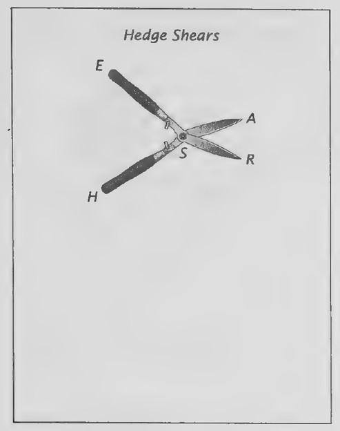Transparency 3-6-3: Hedge shears (Set II, Exs. 40-43)

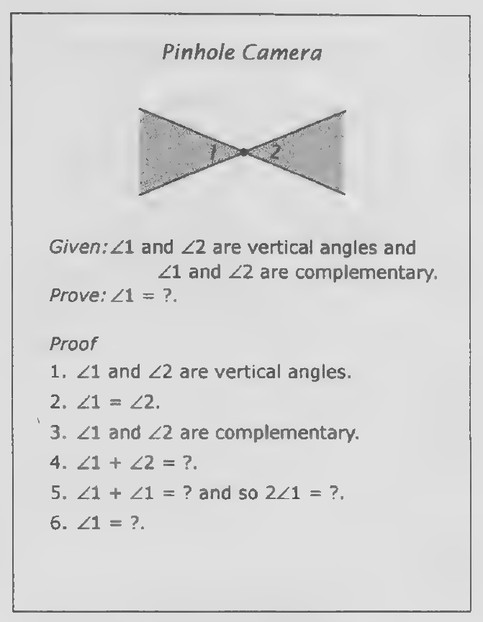Transparency 3-6-4: Pinhole camera (Set II, Exs. 46 and 47)

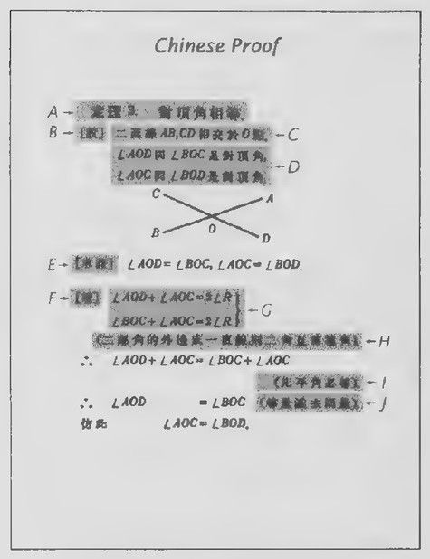Transparency 3-6-5: Chinese proof (Set III)

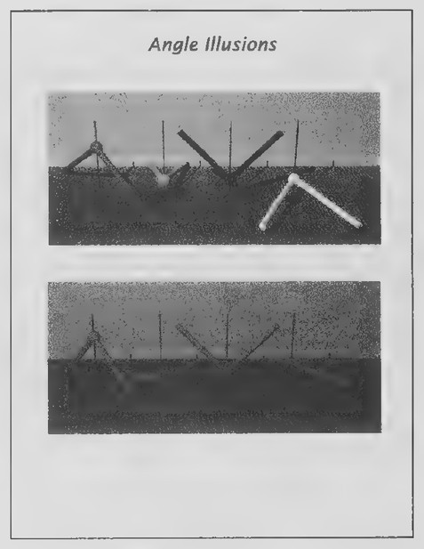Transparency 3-7-1: Angle illusions

Introduction

Transparencies 3-6-1 and 3-6-2 show some terms about angles from a German geometry book. The illustrations on the first transparency name angles according to their measures: Winkel means “angle”; spitze means “pointed” or “acute”; rechte, “right”; stumpfe, “blunt,” “stupid,” or “obtuse”; and gestreckter, “enlongated” or “straight.” The next term names a type of angle that we will not encounter until later: iiberstumpe in German means “beyond stupid” or “beyond obtuse.” Our term for it is “reflex.” The final term refers to the angle through which something turns in making one full revolution: Voll appropriately means “full.”

The terms on the second transparency refer to angle relations: Scheitel means “part,” as in the hair, and neben means “beside.” The caption of the first illustration states that the swinging compass needle produces “scheitelwinkel,” angles that we call vertical. The second illustration shows two positions of a railroad switch, and the caption states that “nebenwinkel,” angles that we called a linear pair, appear in a yield lever. With this introduction, the idea of opposite rays can be introduced, and the rest of the lesson can be developed as in the text.

Lesson 7: Perpendicular and Parallel Lines

Lesson Outline

Terms: Perpendicular, parallel.

Theorem 7. Perpendicular lines form four right angles.

Corollary to the definition of a right angle. All right angles are equal.

Theorem 8. If the angles in a linear pair are equal,

then their sides are perpendicular.

Transparencies

• 3-7-1 Angle illusions
• 3-7-2 A deceptive figure (Set II, Exs. 23-27)

Introduction

The photographs on Transparency 3-7-1 were created by scientists at Duke University and are from Al Seckel’s beautiful book titled The Great Book of Optical Illusions (Firefly Books, 2002). The first photograph shows models of four angles mounted on sticks. Which angle do you think is the largest and which angle do you think is the smallest? (All four angles are right angles!) As Seckel reports: “According to Duke University neuroscientists Dale Purvis,

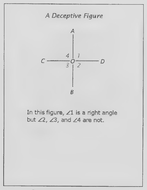Transparency 3-7-2: A deceptive figure (Set II, Exs. 23-27)

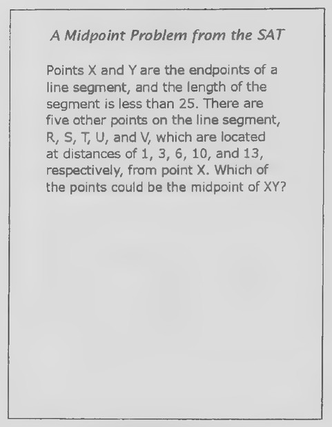Transparency 3-R-1: A midpoint problem from the SAT

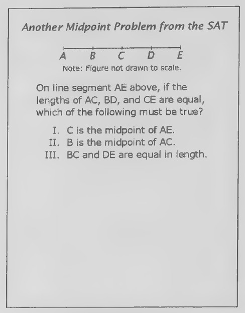Transparency 3-R-2: Another midpoint problem from the SAT

ing to Duke University neuroscientists Dale Purvis, R. Beau Lotto, and Suragit Nundy, the orientation of the angle exerts a strong bias in the judgment of its extent, depending on the frequency of occurrence of particular angles at that orientation in our experience. Angles at the orientation of the red angle tend to be large and [those at the orientation of] the green angle tend to be small, so we overestimate the red as large and we underestimate the green.”

How do the angles in the lower photograph appear to compare in size? (Although they may appear to be right angles and hence equal, they actually differ considerably in size.)*

These questions lead directly into the definition of perpendicular lines and the rest of the new lesson.

Review of Chapter 3

Transparencies

• 3-R-1 A midpoint problem from the SAT
• 3-R-2 Another midpoint problem from the SAT
• 3-R-3 Chair design (Set II, Exs. 37-40)
• 3-R-4 The geometry of a pencil point

First day

Introduction

Transparencies 3-R-1 and 3-R-2 contain two problems that have appeared on SAT tests in the past.

“More on the topic of angle perception can be found in an article titled “Why We See What We Do” in the May-June 2002 issue of American Scientist and in the book of the same name by Dale Purves, Michael A. Wieder, and R. Beau Lotto (Sinauer, 2003).

Both are about midpoints. The first is a good exercise in indirect reasoning and the second, in direct reasoning.

Problem 1. (Suggest that your students draw a figure in which they assign the coordinate 0 to point X. The coordinates of R, S, T, U, and V are 1, 3, 6, 10, and 13, respectively, and the coordinate of Y is less than 25.) Point V cannot be the midpoint of XY, because, if it were, the coordinate of Y would be 26. Point T cannot be the midpoint of XY, because, if it were, the coordinate of Y would be 12; this contradicts the fact that V is on line segment XY. Points R and S are ruled out in the same way; so only U could be the midpoint of XY.

Problem 2. We are given that AC = BD = CE. It immediately follows that AC = CE, and so C is the midpoint of AE. If we imagine that segment BD was moved to the right along the line without changing its length, it is clear that B need not be the midpoint of AC. BC and DE must be equal in length, as the following proof establishes. BD = CE (given). BD = BC+ CD and CE = CD + DE (Betweenness of Points Theorem). So BC + CD = CD + DE (substitution) and BC = DE (subtraction).

Second day

Introduction

Part of the pencil sharpening that goes on in every classroom is due to worn-down pencil leads and part is due to broken pencil points. Many years ago, Don Cronquist, an engineer in California, noticed that almost all broken pencil points have the same size and shape. In analyzing why this should be, Cronquist made drawings similar to the ones on

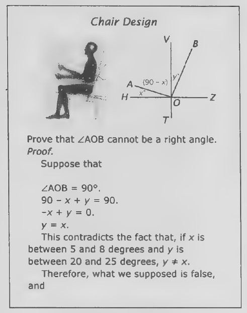Transparency 3-R-3: Chair design (Set II, Exs. 37-40)

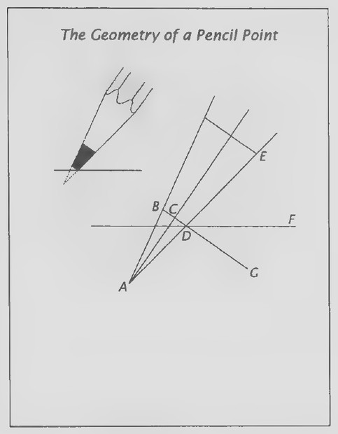Transparency 3-R-4: The geometry of a pencil point

causing pencil points to break; we will look just at the angles in the figure. (This will be easier to do if you hand out duplicated copies of the transparency.) Although a scientist or engineer could use a protractor to measure all of the angles in a given figure, it is usually simpler to start with a few and use geometry to determine the rest. In the lettered figure, AC ∥ BG and AC bisects ∠BAD. Use your protractor to measure ∠BAD, the angle of the cone of the pencil lead, and ∠EDF, the angle of the lead with the paper. (∠BAD = 20°, ∠EDF = 45°.) Now put your protractor aside and see how many of the following angles you can figure out.

1. ∠CAD. (10°, because AC bisects ∠BAD.)

2. ∠ACD. (90°, because AC 1 BG.)

3. ∠CDA. (80°, because it is the third angle in

△CAD. We have just found the measures of

the other two angles and so, from the

Triangle Angle Sum Theorem, we have

∠CDA = 180° — 10° - 90°.)

4. What relation does ∠CDA have to ∠CAD?

(They are complementary.)

5. ∠EDG. (80°, because ∠EDG and ∠CDA are

vertical angles. Vertical angles are equal.)

6. ∠FDG. (35°. DE-DF-DG, and so ∠EDF +

∠FDG = ∠EDG; ∠EDF = 45° and ∠EDG =

80°.)

. ∠ADG. (100°, because ∠ADG and ∠EDG form a linear pair. The angles in a linear pair are supplementary.). ∠BDE. (100°, because ∠BDE and ∠ADG are vertical angles.)

*Don Cronquist’s study of broken pencil points was reported by Jearl Walker in his “Amateur Scientist” column in the February 1979 issue of Scientific American. Henry Petroski also includes it in chapter 3, “Pencil Points and Analysis,” of his book titled Invention by Design—How Engineers Get from Thought to Thing (Harvard University Press, 1996).

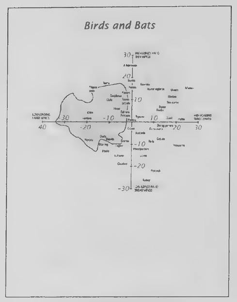Transparency 4-1-3: Bird and bats (Set I, Exs. 16-22)

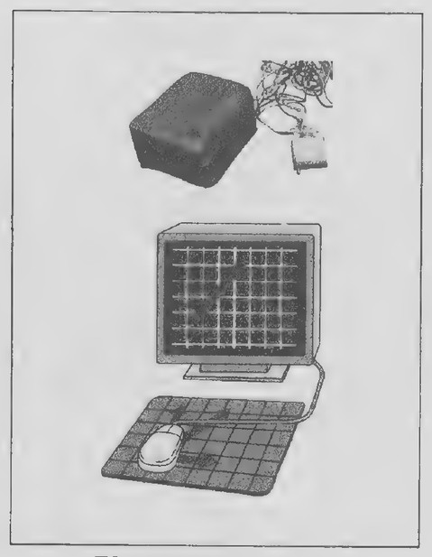Transparency 4-1-1: Computer mouse

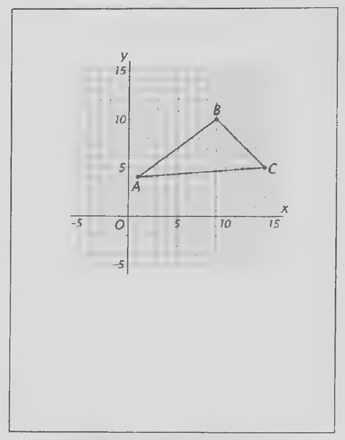Transparency 4-1-2: Triangle and coordinate system

Chapter 4: Congruence

Lesson 1: Coordinates and Distance

Lesson Outline

Terms: Coordinate systems (in one and two dimensions), origin, coordinates, axes, quadrants. The Distance Formula: The distance between the points P,(x,, y,) and P,(x,, y>) is

Vm —-mP +(y-y,).

Transparencies

• 4-1-1 Computer mouse
• 4-1-2 Triangle and coordinate system
• 4-1-3 Bird and bats (Set I, Exs. 16-22)

Introduction

Keeping the rest of Transparency 4-1-1 covered, show the photograph at the top and ask if anyone can identify the object pictured. It is the first computer mouse, built and invented by Douglas Engelbart at the Stanford Research Institute in 1964. Dr. Engelbart called it a mouse “because the tail came out the end,” and in his patent application described it as an “x-y position indicator for a display system.”

Show the figure at the bottom of the transparency. A computer mouse contains a rubber ball that rotates as the mouse is moved. The ball turns two rollers, one to detect horizontal movement and the other to detect vertical movement. This information

is sent by electric signals to the computer, which then moves the cursor on the screen accordingly. All of this is possible because the computer screen operates by a coordinate system.

Show Transparency 4-1-2. In your algebra class, you used coordinate systems to picture linear equations in two variables. You learned that such equations are called linear because they can be graphed as lines. The solutions of a linear equation are pairs of numbers that can be used to locate geometric points. This connection between the numbers of algebra and the points of geometry works both ways. For example, the properties of this triangle can be studied by assigning pairs of numbers to its corners. Add the overlay to the transparency and guide your students in using the resulting coordinates to make an accurate copy of the figure on a sheet of graph paper. [Note: Tape the overlay to the transparency so that the coordinates of the vertices of the triangle are A(1, 4), B(9, 10), and C(14, 5).] The basic ideas of the lesson can be introduced as your students copy the figure. After developing the Distance Formula, apply it to finding the lengths of the sides of the triangle in terms of the unit used in the coordinate system. That the calculated lengths are reasonable can be verified by marking the edge of a file card with the units of the graph paper so that it can be used as a ruler to put in place along the sides of the triangle. (AB = 10, BC = 150 ~7.1, AC = 130 = 11.4.)

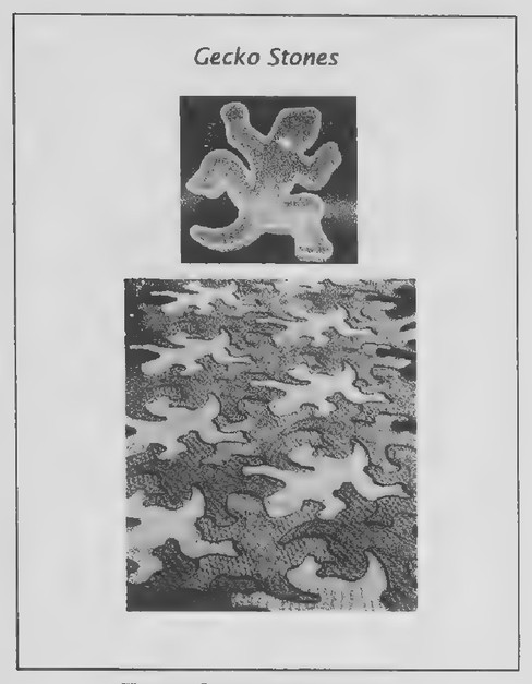Transparency 4-2-1: Gecko stones

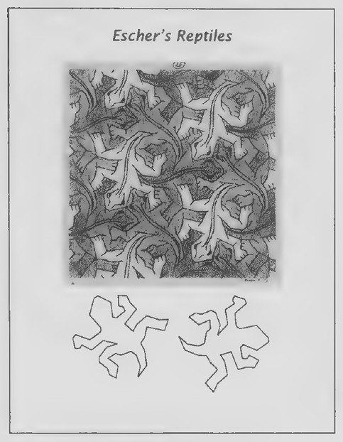Transparency 4-2-2: Escher’s reptiles

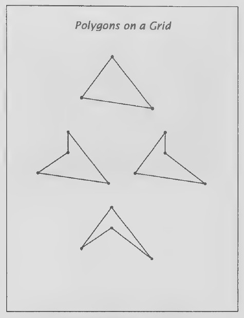Transparency 4-2-3: Polygons on a grid (Set II, Exs. 44-47)

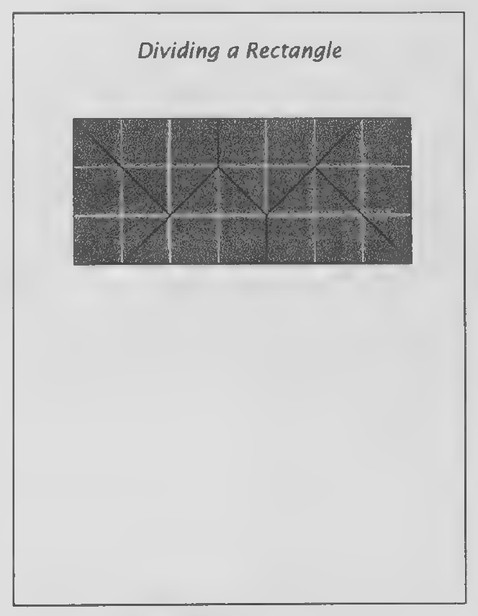Transparency 4-2-4: Dividing a rectangle (Set II, Exs. 48-54)

Lesson 2: Polygons and Congruence

Lesson Outline

Terms: Polygon, sides, vertices, congruent figures, congruence correspondence.

Definition: Congruent triangles.

Corollary to the definition of congruent triangles. Two triangles congruent to a third triangle are congruent to each other.

Transparencies

• 4-2-1 Gecko stones
• 4-2-2 Escher’s reptiles
• 4-2-3 Polygons on a grid (Set II, Exs. 44-47)
• 4-2-4 Dividing a rectangle (Set II, Exs. 48-54)

Introduction

The photograph at the top of Transparency 4-2-1 shows a mold for making concrete paving stones in the shape of geckos, lizards found throughout the Hawaiian Islands. Created by John August, an architectural designer based in Maui, the stones can be interlocked with one another to pave walkways, as shown in the photograph at the bottom. (More on August’s designs can be found on the following Web site: www.geckostone.com.)

August’s paving stones are based on a drawing created by Maurits Escher. In contrast to the curved border of August’s gecko figure, Escher’s reptiles are bordered by line segments. For this reason, they are polygons. The lesson can now be developed as in the text. (Escher’s reptile polygon is a 50-gon. The two copies of it at the bottom of Transparency 4-2-2 are for use in introducing the idea of a congruence correspondence.)

Lesson 3: ASA and SAS Congruence

Lesson Outline

Terms: Included and opposite sides and angles.

Postulate 5. The ASA Postulate. If two angles and the included side of one triangle are equal to two angles and the included side of another triangle, the triangles are congruent.

Postulate 6. The SAS Postulate. If two sides and the included angle of one triangle are equal to two sides and the included angle of another triangle, the triangles are congruent.

Transparencies

• 4-3-1 Artillery triangle
• 4-3-2 Example proof 1

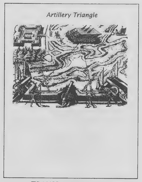Transparency 4-3-1: Artillery triangle

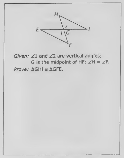
Transparency 4-3-2: Example proof 1

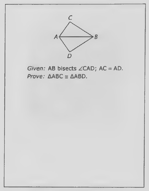
Transparency 4-3-3: Example proof 2

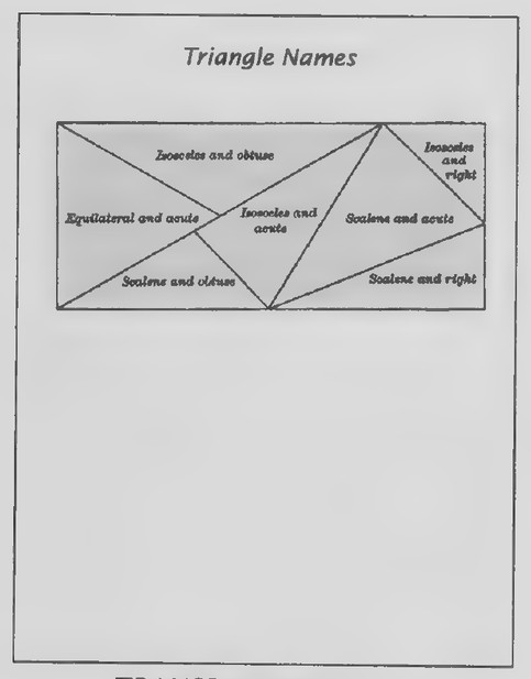Transparency 4-3-4: Triangle names (Set I, Exs. 16-21)

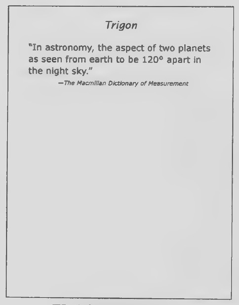Transparency 4-3-5: Trigon

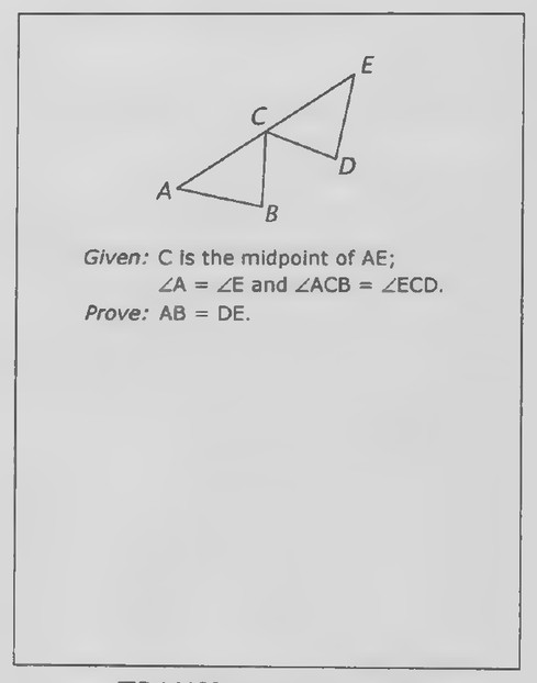Transparency 4-3-6: Example proof 3

• 4-3-3 Example proof 2
• 4-3-4 Triangle names (Set I, Exs. 16-21)
• 4-3-5 Trigon
• 4-3-6 Example proof 3
• 4-3-7 Example proof 4

First day

Introduction

The figure on Transparency 4-3-1, from a book published in 1648, shows a cannon aimed at a target. Two people on either side of the cannon are shown measuring angles at the base of a large triangle to figure out the distance to the target. To see how the method works, we will draw a comparable figure. Suppose that the two angle measurers are 80 yards apart. Draw a horizontal line segment AB 4 inches

long to represent this distance. How many yards does 1 inch along AB represent? (20.) Suppose that the person at A measures an angle of 60° between AB and the line of sight to the target. Center your protractor at A and draw a line forming a 60° angle with AB. Suppose that the person at B measures an angle of 75° between AB and the line of sight to the target. Center your protractor at B and draw a line forming a 75° angle with AB. The point in which the two lines intersect marks the location of the target; label it C. Notice that the shape of △ABC is determined by the length of side AB and the measures of the two angles at its endpoints, ∠A and ∠B. Suppose that the cannon is located midway between A and B. Use your ruler to measure the distance from

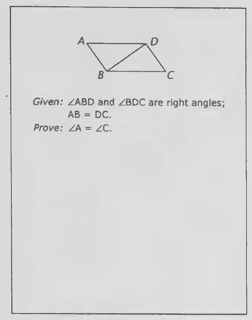Transparency 4-3-7: Example proof 4

Transparency 4-4-1: The cowboys and the drive-in

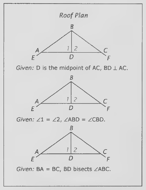Transparency 4-4-2: Roof plan (Set I, Exs. 1-17)

the cannon to the target. (About 4.75 in.) Approximately how many yards is it from the cannon to the target? (4.75 x 20 = 95 yd.)

Point out that, in drawing the artillery triangle, we did not need to know the lengths of all three of its sides and the measures of all three of its angles. The rest of the lesson can now be developed as in the text.

Transparencies 4-3-2 and 4-3-3 are for use in providing your students practice in proving triangles congruent.

Second day

Introduction

Show Transparency 4-3-5. The word “trigon” is another word for “triangle,” although it is seldom used anymore. According to The Macmillan Dictionary of Measurement (Macmillan, 1994), “trigon” has also been used in astronomy to mean “the aspect of two planets as seen from earth to be 120° apart in the night sky.”

Have your students use their protractors to draw a 120° angle. Label its vertex E to represent the position of the earth. Now suppose that Jupiter and Saturn are seen along the sides of this angle when their distances from earth are 400,000,000 miles and 950,000,000 miles, respectively. For convenience, we will let 1 cm represent 100,000,000 miles. Mark point J to represent Jupiter on one side of ∠E so that EJ = 4 cm. Mark point S to represent Saturn on the other side of ∠E so that ES = 9.5 cm. Draw and measure segment JS. How far apart are Jupiter and Saturn at this time? (JS =~ 12 cm; so the distance between Jupiter and Saturn is about

1,200,000,000 miles.) Notice that the shape of △JES is determined by the measure of ∠E and the lengths of the two sides EJ and ES. Why is it reasonable to expect that all triangles drawn with these same measurements would be congruent? (They would be congruent by the SAS Congruence Postulate.)

Transparencies 4-3-6 and 4-3-7 are for use in providing your students practice in proving triangles congruent and that corresponding parts of them are equal.

Lesson 4: Congruence Proofs

Lesson Outline

Definition (brief restatement for congruent triangles): Corresponding parts of congruent triangles are equal.

Transparencies

• 4-4-1 The cowboys and the drive-in
• 4-4-2 Roof plan (Set I, Exs. 1-17)
• 4-4-3 . Congruence proof (Set II, Ex. 30)
• 4-4-4 Congruence proof (Set II, Ex. 31)
• 4-4-5 Congruence proof (Set II, Ex. 32)
• 4-4-6 Congruence proof (Set II, Ex. 33)
• 4-4-7 Grid exercise (Set II, Exs. 34-46)

Introduction

The figure on Transparency 4-4-1 is for use in presenting Lesson 4 as in the text. The proof that the procedure works is another example of proving triangles congruent and using the definition of congruent triangles to conclude that their corresponding parts are equal. If you direct your students in

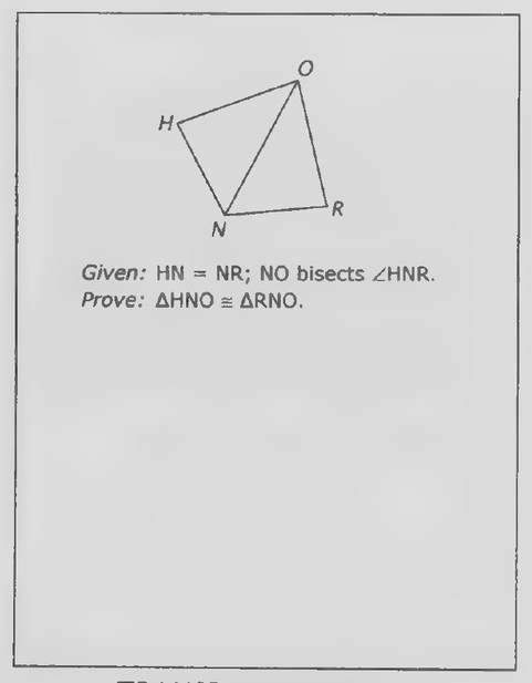Transparency 4-4-3

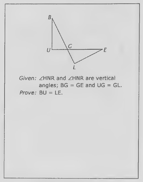Transparency 4-4-4: Congruence proof (Set II, Ex. 31)

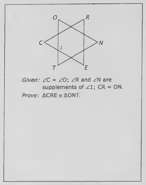Transparency 4-4-5: Congruence proof (Set II, Ex. 32)

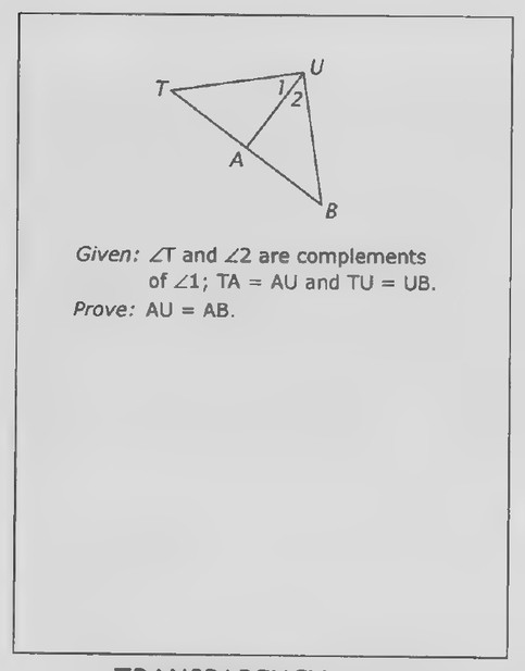Transparency 4-4-6: Congruence proof (Set II, Ex. 33)

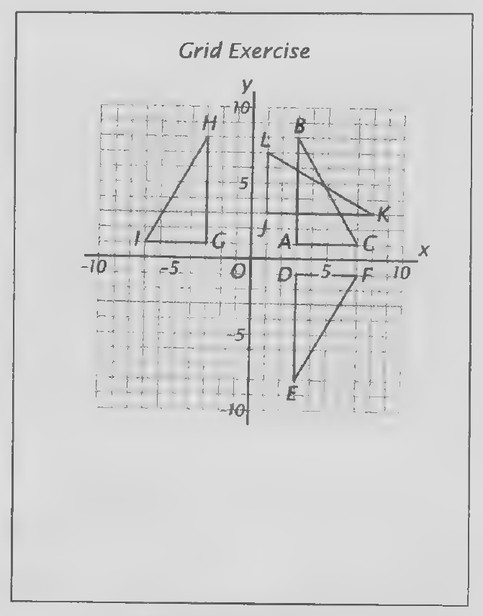Transparency 4-4-7: Grid exercise (Set II, Exs. 34-46)

Transparency 4-5-1: Triangle challenge

writing this proof in their notes, it is best to state the “given” as in the text to ensure that the proof is reasonably straightforward. A method comparable to the one for finding the distance to the drive-in may have been used by the Babylonians and Egyptians for measuring the distances of ships from the shore.

Lesson 5: Isosceles and Equilateral Triangles

Lesson Outline

Terms: Types of triangles: scalene, isosceles, equilateral, obtuse, right, acute, equiangular.

Theorem 9. If two sides of a triangle are equal, the angles opposite them are equal.

Corollary to Theorem 9. An equilateral triangle is

equiangular. Theorem 10. If two angles of a triangle are equal,

the sides opposite them are equal. Corollary to Theorem 10. An equiangular triangle is

equilateral.

Transparencies

• 4-5-1 Triangle challenge
• 4-5-2 Theorem 10 (Set II, Ex. 33)
• 4-5-3 Corollary to Theorem 10 (Set II, Ex. 35)
• 4-5-4 Star puzzles (Set II, Exs. 43-47)
• 4-5-5 Drawing exercise (Set II, Exs. 49-53)

Introduction

Hand out duplicated copies of Transparency 4-5-1. This triangle once appeared in the “Mathematical

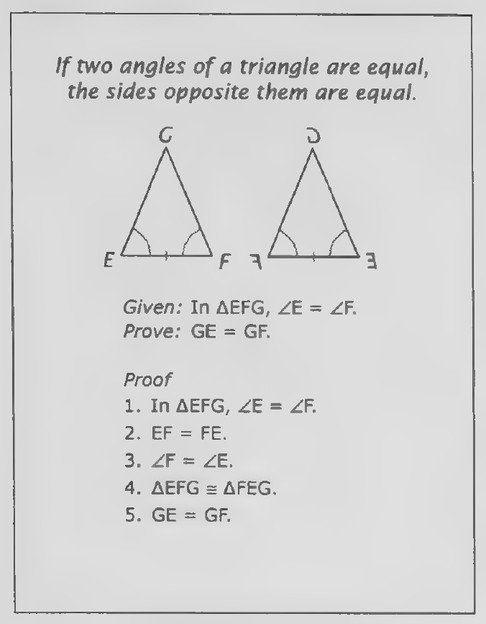Transparency 4-5-2: Theorem 10 (Set II, Ex. 33)

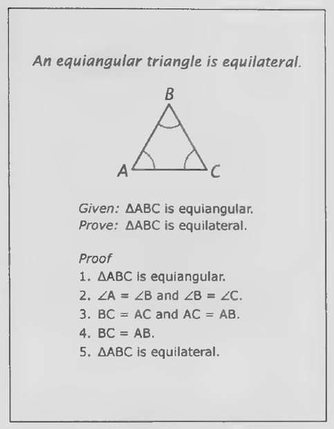Transparency 4-5-3: Corollary to Theorem 10 (Set II, Ex. 35)

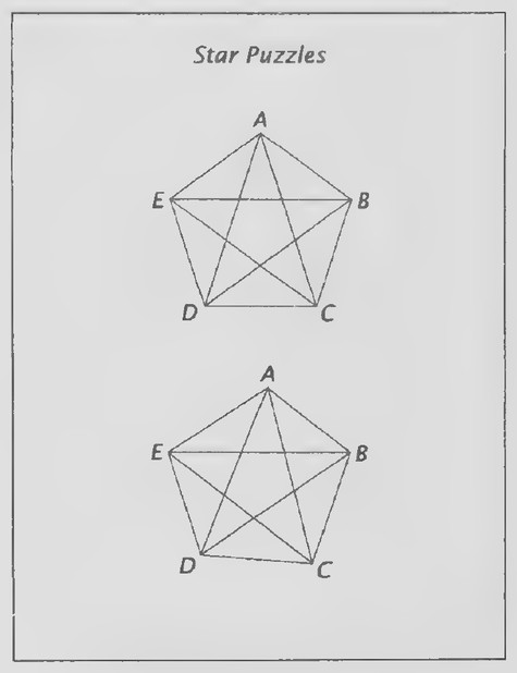Transparency 4-5-4: Star puzzles (Set II, Exs. 43-47)

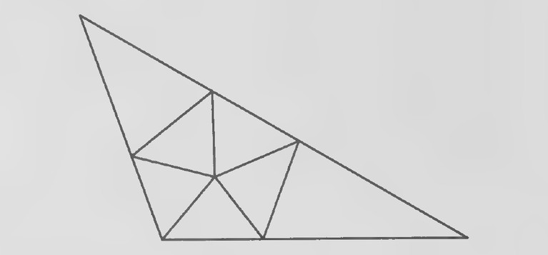Figure on page 323

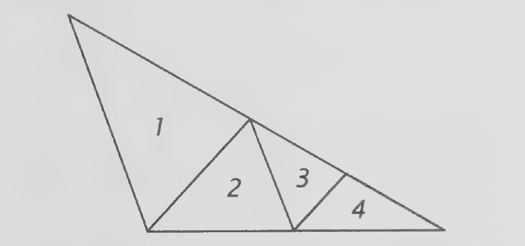Figure on page 323

Games” column of Scientific American (February 1960). Ask your students to use their protractors to measure its largest angle. (110°.) Explain that this triangle is said to be “obtuse” because it has an obtuse angle, in contrast with a “right” triangle, which has a right angle, and an “acute” triangle, all of whose angles are acute.

The challenge in the magazine was to divide the obtuse triangle into smaller triangles, all of which are acute. As an example of an attempt to do so, add lines to the triangle on the transparency as shown in the following figure.

VSS

three triangles are acute, the fourth is obtuse, and so these lines do not solve the problem. Give your students a few minutes to try to find a solution. (You might even offer a small prize to the first student to do so.) It is unlikely that anyone will be able to solve the problem very quickly. You might want to leave the problem dangling for a few days. If so, you might suggest it as something to work on in other classes, if you get bored!

In the book in which the “Mathematical Games”

column containing this problem was reprinted, Martin Gardner reported that “A number of readers [of Scientific American] sent ‘proofs’ that an obtuse triangle cannot be dissected into acute triangles, but of course it can. The following figure shows a seven-piece pattern that applies to any obtuse triangle.”

Gardner triangles are necessary. The obtuse angle has to be divided by a line. If this line goes all the way to the other side, it will form either another obtuse angle or right angles, all of which would also have to be divided. So the line dividing the obtuse angle has to stop at some point inside the triangle. For all of the angles from this point to be acute, at least five lines have to be drawn. (Four lines would form four angles, but they cannot all be acute, because four numbers each less than 90 cannot add up to 360.) The result is an “inner pentagon” of five triangles, resulting in seven triangles altogether. Gardner also reported that it was a Brooklyn high-school student at the time, Wallace Manheimer, who figured out this proof. It was published in the American Math-

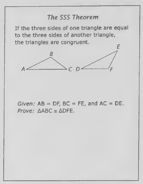Transparency 4-6-2: The SSS theorem

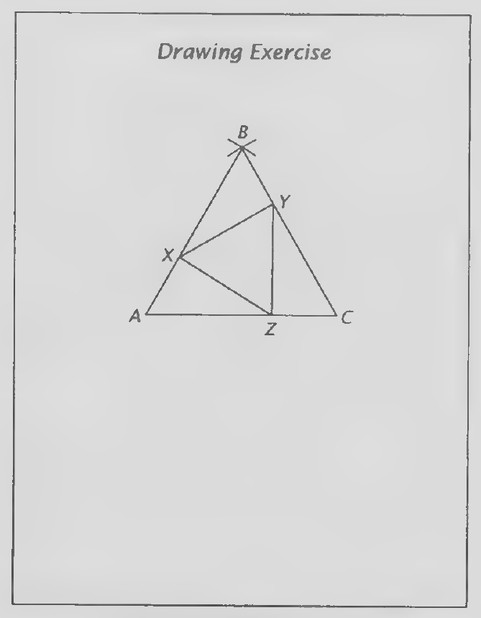Transparency 4-5-5: Drawing exercise (Set II, Exs. 49-53)

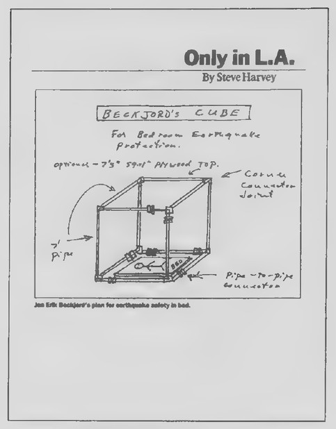Transparency 4-6-1: Beckjord’s cube

ematical Monthly.

In trying to find a solution to this problem, our attention is drawn to the angles of triangles. At the same time, we have seen that triangles are classified according to their angles. They are also classified according to their sides. The rest of the lesson can now be developed as in the text. Theorem 9, known as the Isosceles Triangle Theorem, has an interesting history. The faces of the pyramids have the shape of isosceles triangles, and the Egyptians undoubtedly knew as far back as 2700 B.C. that, if two sides of a triangle are equal, the angles opposite them also must be equal. The Greek mathematician Thales, born in 625 B.C., is thought to have learned geometry in his travels to Egypt and may have been the first to prove the Isosceles Triangle Theorem. Euclid, who lived about 300 years later, included the theorem in his Elements. The proof of the theorem considered in the text is simpler than Euclid’s and is attributed to Pappus, a Greek geometer who lived in Alexandria in about 300 a.p. When computer programs were first developed to prove geometrical theorems in 1956, acomputer came up with the very same proof! Some comments by Marvin Minsky about the computer proof can be found on the following Web site: www.math. niu.edu/~rusin/known-math/99/minsky.

Lesson 6: SSS Congruence

Lesson Outline

Theorem 11. The SSS Theorem. If the three sides of one triangle are equal to the three sides of

another triangle, the triangles are congruent.

Transparencies

• 4-6-1 Beckjord’s cube
• 4-6-2 The SSS theorem
• 4-6-3 Plumb level (Set I, Exs. 3-8)
• 4-6-4 Linkage problem 1 (Set II, Exs. 26-35)
• 4-6-5 Linkage problem 2 (Set II, Exs. 36-43)
• 4-6-6 Grid exercise (Set II, Exs. 44-51)
• 4-6-7 Bracing the square (Set III)

Introduction

Not long after the big earthquake in Los Angeles in 1994, the figure on Transparency 4-6-1 was published in the Los Angeles Times (February 3, 1994). According to the article with which it appeared, actor Jerry Van Dyke had survived the quake because of a four-posted bed that propped up the falling ceiling of his bedroom. This gave Jon Erik Beckjord the idea of developing a cube made out of pipes for bedroom earthquake protection. Beckjord claimed that the thicker the pipe, the more secure the bed inside the cube would be.

A dramatic illustration that such a cubical structure, consisting only of squares, is not rigid would be to show one made of drinking straws threaded together. A second structure to which a diagonal has been added to each face is rigid because the shape of the resulting triangles, unlike that of the squares, is determined by the lengths of their sides.

For convenience in developing the proof of the SSS Theorem, I suggest handing out duplicated copies of Transparency 4-6-2. Direct your students in using their protractor and ruler to copy △DEF below △ABC as done in the text. There is room on the

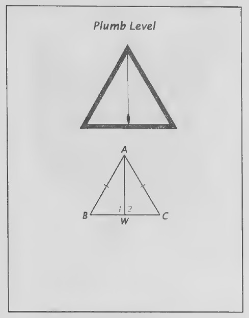Transparency 4-6-3: Plumb level (Set I, Exs. 3-8)

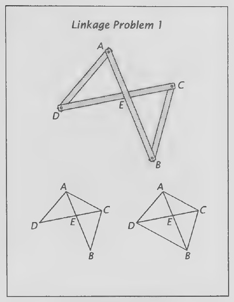Transparency 4-6-4: Linkage problem 1 (Set II, Exs. 26-35)

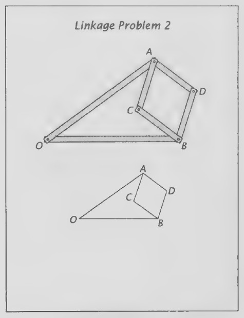Transparency 4-6-5: Linkage problem 2 (Set II, Exs. 36-43)

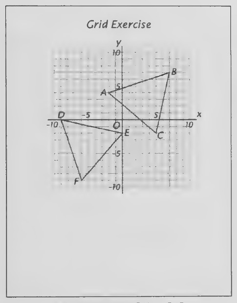Transparency 4-6-6: Grid exercise (Set II, Exs. 44-51)

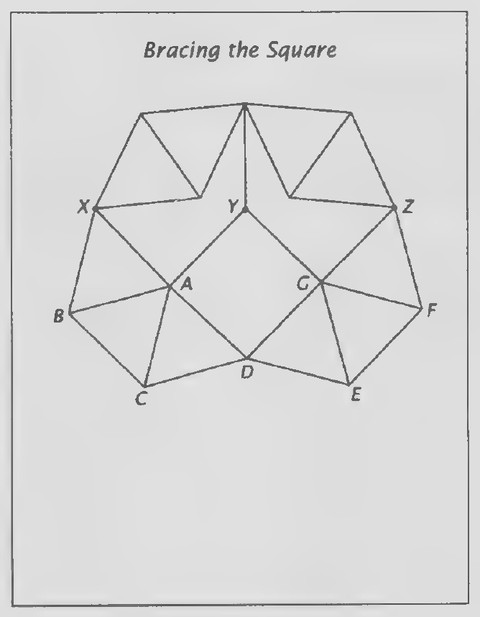Transparency 4-6-7: Bracing the square (Set III)

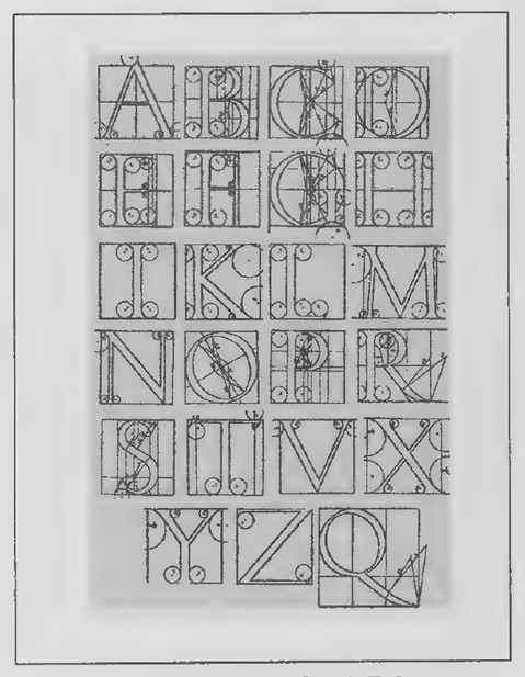Transparency 4-7-1: Torniello’s alphabet

lower part of the transparency to outline the main ideas of the proof. When you have finished, be sure to let your students know that you hope they have understood how the proof works but that you do not expect them to remember all of the details. The goal here might be compared to understanding the structure of a poem rather than having to memorize it.

Lesson 7: Constructions

Lesson Outline

Construction 3. To copy a line segment.

Construction 4. To copy an angle.

Construction 5. To copy a triangle.

Transparencies

• 4-7-1 Torniello’s alphabet
• 4-7-2 Car jack (Set I, Exs. 22-29)
• 4-7-3 . An unexpected result (Set II, Exs. 30-33)

Introduction

In the Renaissance, several attempts were made to apply mathematics to designing the letters of the alphabet.* The Italian mathematician Luca Pacioli included an appendix on alphabets in a book on geometry published in 1509. Another Italian, the type designer Francesco Torniello, published a book titled The Alphabet in 1517 in which he showed how

*TEX and METAFONT —New Directions in Typesetting, by Donald E. Knuth (Digital Press, 1979).

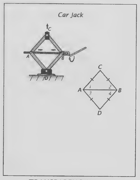Transparency 4-7-2: Car jack (Set I, Exs. 22-29)

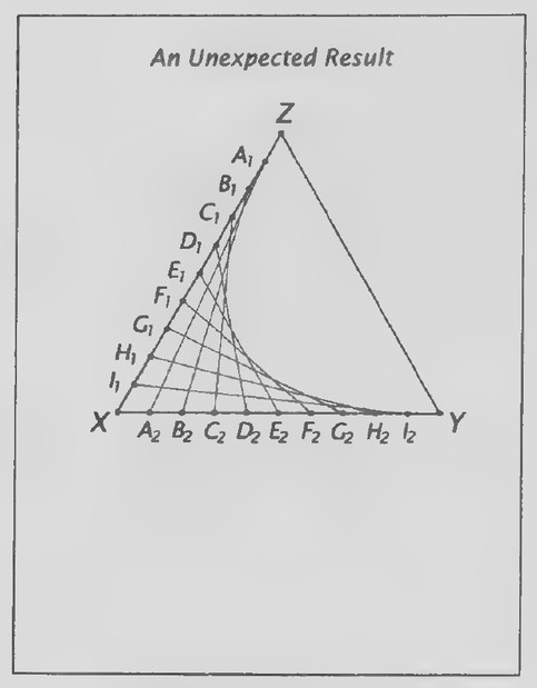Transparency 4-7-3: An Unexpected Result

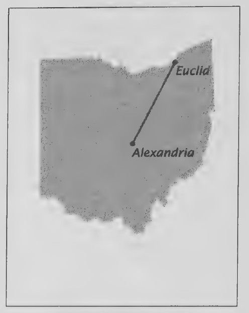Transparency 4-R-1: Euclid to Alexandria

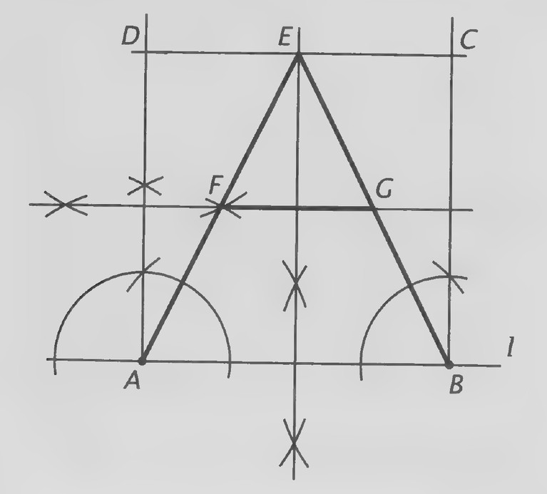Figure on page 326 — Construction diagram with a rectangle ABCD, a triangle ADE, equal arcs from A and B, and points F and G

to construct capital letters with straightedge and compass. The figures on Transparency 4-7-1 are from Torniello’s book. The outline of each letter consists of line segments, drawn with a straightedge, and arcs of circles, drawn witha compass.

Remind your students that it was Euclid who established the use of the straightedge and compass for making geometric constructions at the very beginning of his Elements. We constructed an equilateral triangle at the beginning of the course, and we have learned how to bisect both line segments and angles. In this lesson, we will learn how to make three more basic constructions. One way to introduce them would be to construct a simple version of a capital A as shown in the following figure and

described in the steps that follow. (Note that the steps review the bisection constructions, as well as introducing the new ones; so demonstrate them at the overhead projector as you lead your students through them. There is no need tojustify results such as the formation of the four squares.)

1. Draw a horizontal line / and choose a point A

on it. 2. Bisect straight ∠A to form two right angles. 3. Choose a second point B on! approximately

3 inches to the right of A. 4. Construct a right angle at B by copying one

of the right angles at A.

. Copy segment AB to get AD and BC. O1 Oo. Bisect AB and AD to divide the square into

four smaller squares. 7. Label point E and draw EA and EB. Also

draw the cross bar of the capital A and label

its endpoints F and G.

Is △ABE equilateral? (No.) Show your students how to copy the capital A ina different place on the paper by first copying △ABE and then copying AF and BG to determine FG.

Review of Chapter 4

Transparencies

• 4-R-1 Euclid to Alexandria
• 4-R-2 Toll rate distances
• 4-R-3 Ollie’s mistake (Set II, Exs. 37-42)
• 4-R-4 Proof (Set II, Ex. 51)
• 4-R-5 Proof (Set II, Ex. 52)
• 4-R-6 Euclid carved in stone
• 4-R-7 Euclid’s Elements

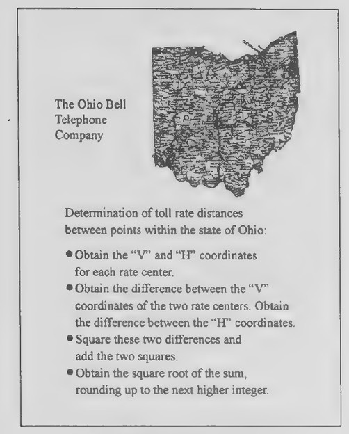Transparency 4-R-2: Toll rate distances

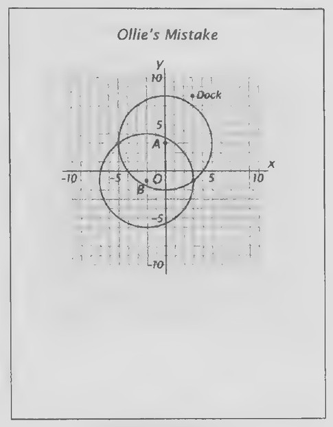Transparency 4-R-3: Ollie’s mistake (Set II, Exs. 37-42)

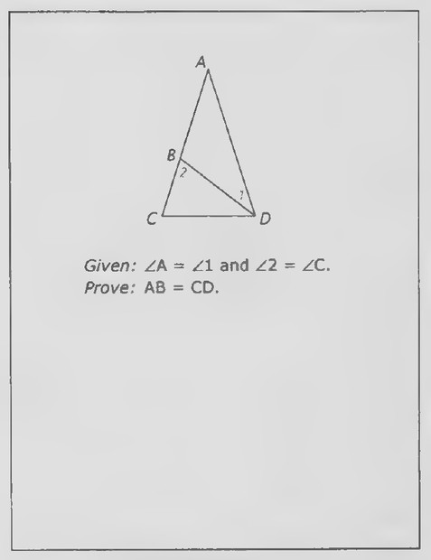Transparency 4-R-4: Proof (Set II, Ex. 51)

First day

Introduction

It might seem impossible for Euclid to place a call to Alexandria, but it could happen in Ohio! Euclid is a city on the shore of Lake Erie, northeast of Cleveland (Transparency 4-R-1). It was named, as you might suspect, for the Greek mathematician. Alexandria, asmall town located near the center of Ohio, is named for the city in Egypt where Euclid lived.

To calculate the toll rate for a call between two points in Ohio, the Ohio Bell Telephone Company applies a series of rules, part of which are listed on Transparency 4-R-2. Even though you have never seen these rules before, they may seem familiar. Why? (They sound like the Distance Formula.) As the Web site of the Telco Exchange explains, “The Telecom industry has its own unique system of geography. Pricing for many services is based on the ‘airline mileage’ or special distance calculations between points. A unique vertical and horizontal (V&H) coordinate system was developed by AT&T Long Lines in 1960 for the North American continent that is used to define telecom locations. The conventional system of longitude and latitude for describing geographic locations is not used. Although based on the well-known Pythagorean Theorem for calculating distances between points on an X-Y coordinate system, the telecom calculations must be made using a litany of special rules and rounding conventions….”*

As a review of the derivation of the Distance Formula from the Pythagorean Theorem, have your

students mark two points, A and E, on paper to represent Alexandria and Euclid. Label the coordinates of A(V₁, H₁) and the coordinates of E(V₂, H₂). Draw a horizontal line through A and a vertical line through E to form right △ABE. In the distance calculation, what do the differences between the respective coordinates represent? (The lengths of the legs of the triangle.) The V&H coordinates for Euclid and Alexandria are (5536, 2527) and (5915, 2513), respectively. How does the V-H coordinate system seem to differ from our x-y coordinate system? (In our x-y coordinate system, the horizontal coordinate is listed first, whereas in the V-H system, the vertical coordinate is listed first. Also, in the V-H system, the vertical coordinates decrease as you proceed upward.) Use the coordinates of A and B to find the “lengths” of AB and BE. (AB = 2527 − 2513 = 14; BE = 5915 − 5536 = 379.) Use the Pythagorean Theorem to find the “length” of AE. (AE² = AB² + BE²; so AE² = 379² + 14² = 143,641 + 196 = 143,837 and AE = √143,837 ≈ 380.) The distance between Alexandria and Euclid is 120 miles. Roughly how does the length of one unit in the V-H system compare with 1 mile? (It is about one-third of a mile.)

Second day

Introduction

The photographs on Transparency 4-R-6 are of windows in a monastery in Switzerland. The windows date at about 1320 and are examples of geometric tracery, ornamental stone work of interlaced lines and arcs. Their designer was clearly influenced by the constructions of geometry. In an article titled

*www.telcoexchange.com /resources/ carriers/distance.shtml

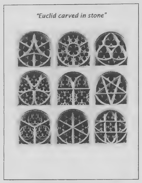Transparency 4-R-6: Euclid carved in stone

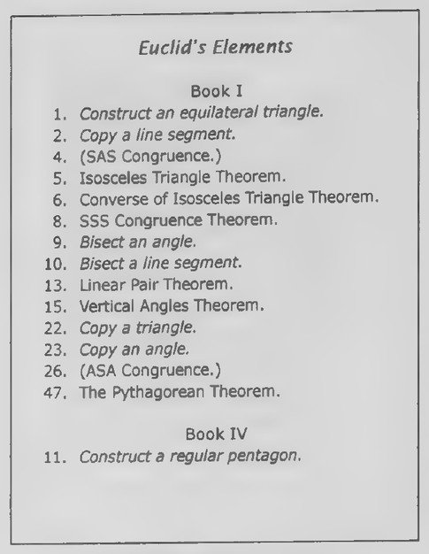Transparency 4-R-7: Euclid’s Elements

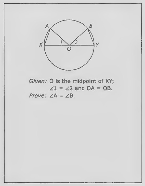Transparency 4-R-5: Proof (Set II, Ex. 52)

“The Cloisters of Hauterive” (pronounced Oh-tereef) in The Mathematical Intelligencer (Spring 1991), Benno Artmann describes the theme of the windows as “geometry itself” and described the windows themselves as “a commentary to Euclid… carved in stone.”* Several windows contain designs that are related to the equilateral triangle; the first and third windows of the first row are especially obvious examples. Which windows seem to contain squares? (The second window of the second row; the last window of the third row.) Which window seems to contain the most polygons? (The last window of the second row.) What polygons do you see init? (Five small acute isosceles triangles and a small pentagon, five overlapping obtuse isosceles triangles, five overlapping kite-shaped quadrilaterals. There are also five overlapping concave pentagons as well as a concave decagon, but I suggest that you mention these polygons only if your students happen to notice them.) We will look at one way to construct the basis pattern of this window, but first we will see where it fits into Euclid’s Elements.

Some of the statements in the first and fourth books (chapters) of the Elements are shown on Transparency 4-R-7 (and listed here). Euclid called the statements “propositions”; we call them “constructions” and “theorems.”

Book I

1. Construct an equilateral triangle.

2. Copy a line segment.

(SAS Congruence.)

Isosceles Triangle Theorem.

Converse of Isosceles Triangle Theorem.

SSS Congruence Theorem.

9. Bisect an angle. 10. Bisect a line segment. 13. Linear Pair Theorem. 15. Vertical Angles Theorem. 22. Copy a triangle. 23. Copy an angle. 26. (ASA Congruence.) 47. The Pythagorean Theorem. Book IV 11. Construct a regular pentagon.

This list might provide a good basis for review. The italicized propositions are the constructions with which your students are now acquainted. The parenthetical propositions indicate that Euclid proved both SAS and ASA congruence as theorems; we treated these statements as postulates. The designer of the windows went well beyond the first book of the Elements. It was not until Book IV that Euclid showed how to construct a regular pentagon. (Explain that a regular pentagon, like an equilateral triangle, has equal sides and angles.) If the lines of the sides of a regular pentagon are extended until they intersect, they form a five-pointed star called a pentagram. This figure is the pattern of the window that we will now construct.

Give your students the following directions so that they can construct the figure as you demonstrate the steps either at the blackboard or on the

*Material on the mathematics of the Cloisters of Hauterive can be found on the following Web site: www.maths.adelaide.edu.au/pure/ pscott/place/pm13/pm13

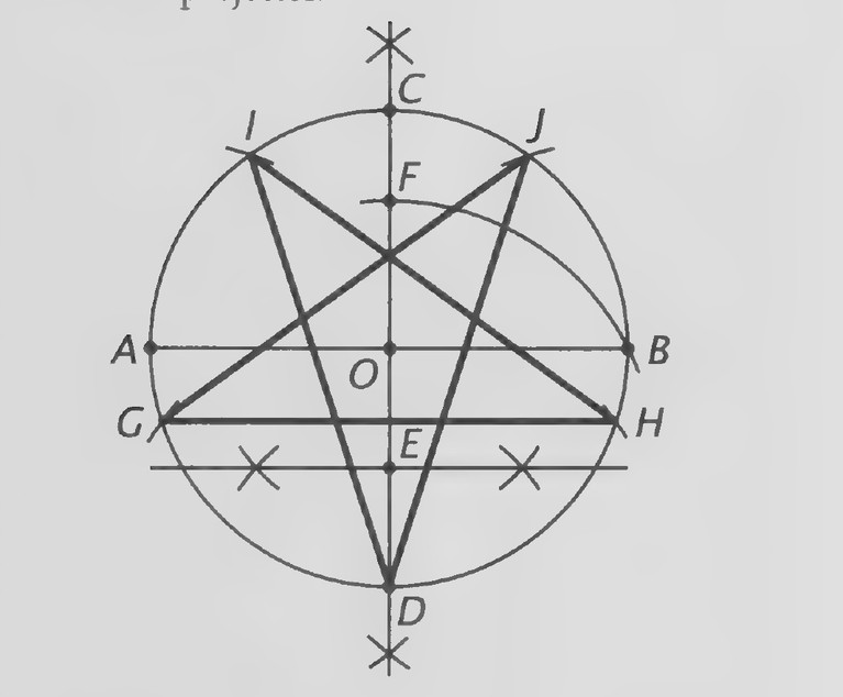Figure on page 329 — A regular pentagon inscribed in a circle with all its diagonals drawn, forming a pentagram (points A–J marked)

overhead projector.

long. 2. Bisect AB and label its midpoint O. 3. Mark points C and D on the bisecting line so

that OC = OD = OA. 4. Bisect OD and label its midpoint E. 5. With E as center and EB as radius, draw an

arc intersecting CD at F. 6. Draw circle O with radius OA. 7. With D as center and BF as radius, draw arcs

intersecting circle O at G and H. 8. With G and H as centers and BF as radius,

draw arcs intersecting circle O at I and J. 9. Draw the pentagram by drawing the seg-

ments DI, IH, HG, GJ, and JD.

After your students have completed the construction, show Transparency 4-R-6 so that they can see the pentagram window again. Explain that, although we have carried out the steps in constructing the pentagram correctly, we are not yet in position to know why they work. This part of our understanding of geometry will come later in the course.

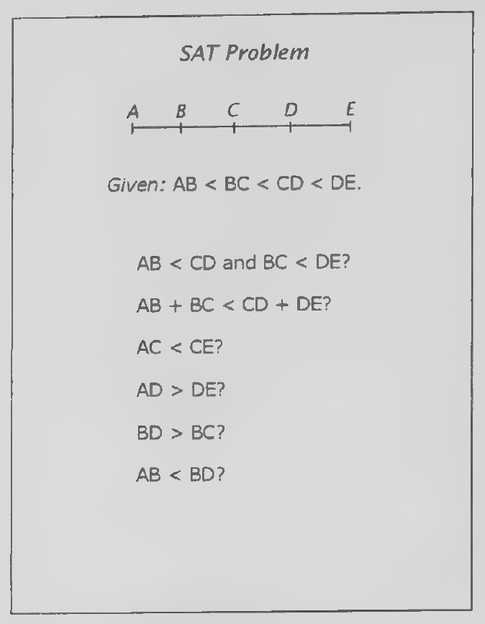Transparency 5-1-3: SAT problem (Set II, Exs. 26-31)

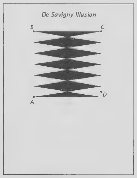Transparency 5-1-1: De Savigny illusion

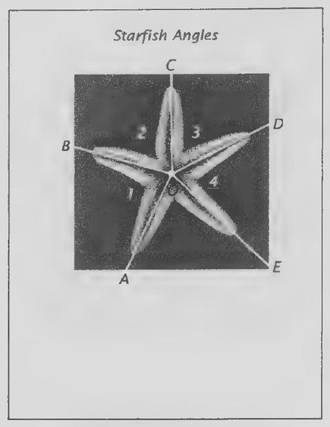Transparency 5-1-2: Starfish angles

Chapter 5: Inequalities

Lesson 1: Properties of Inequality

Lesson Outline

Properties of inequality: “Three possibilities,” transitive, addition, subtraction, multiplication, division, addition theorem, “whole greater than part” theorem.

Transparencies

• 5-1-1 De Savigny illusion
• 5-1-2 Starfish angles
• 5-1-3 SAT problem (Set II, Exs. 26-31)
• 5-1-4 Proof (Set II, Ex. 48)

Introduction

The figure on Transparency 5-1-1 is based on one from a book published in France in 1905 titled The Entertainments of Science.* Four points have been added to the figure for reference. How do you think the distance from A to B compares with the distance from B to C² (You might poll your class on this question by a show of hands. After doing so, use a transparent ruler to measure the two distances. AB appears to be about 4 inches and BC almost a quarter inch longer.)

So far in our study of geometry, we have paid most of our attention to line segments and angles

that are equal. We now turn to comparisons of line segments and angles that are not equal. To do so, we need to make some new assumptions. For example, in comparing the distances AB and BC in the illusion of Transparency 5-1-1, we took for granted that there were only three possibilities. Either AB > BC, AB = BC, or AB < BC. It is reasonable to think that no other possible relations between the two lengths might exist. We will assume that this is so and call it the three possibilities property of inequality.

Here is an example of another property of inequality. It is easy to see from the figure that AB > CD. From this observation and the fact that BC > AB, we can figure out how BC and CD compare in length without doing any more measuring. What conclusion can you draw? (Because BC > AB and AB > CD, BC > CD.) This conclusion is based on the transitive property of inequality.

We need to also include the operations of addition, subtraction, multiplication, and division in our list of properties of inequality. You are already familiar with these properties from your study of algebra. (As a quick review of them, you might ask your students to verbally solve each of the following equation-and-inequality pairs.)

1S B= 74 = 10)

2. X=3 = 72@:<110))

3. A+ x= 9) (eS 5,)

4, 44+x>9.(x>5,)

*In the book, by G. B. De Savigny, the figure was drawn so that AB = BC. The figure is a variation of the “Oppel illusion” and is discussed on page 140 of Jacques Ninio’s book titled The Science of Illusions (Cornell University Press, 2001).

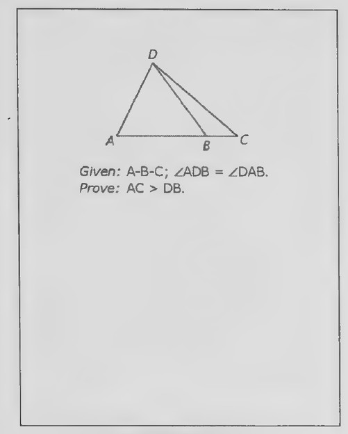Transparency 5-1-4: Proof (Set II, Ex. 48)

Transparency 5-2-1: A photograph of a UFO?

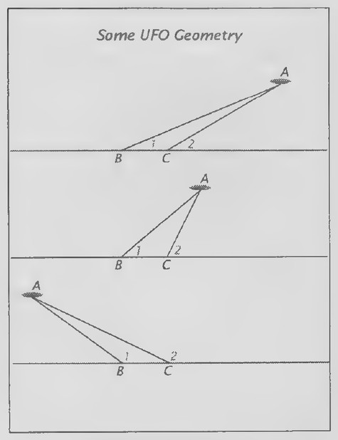Transparency 5-2-2: Some UFO Geometry

6. = 5 < & (x (x < 16. )

Tink = OO, (x =’6,)

Soc 30.10 S26!)

Transparency 5-1-2 is for possible use in introducing the two properties of inequality that are proved in this lesson: the Addition Theorem of Inequality and the “Whole Greater than Part” Theorem.

The angles between the arms of a starfish vary from one starfish to another. In the starfish shown in the photograph, 21 > 23 and 22 > 24. Given this information, how do you think ∠AOC and ∠COE compare in size? (∠AOC > ∠COE.) This conclusion is based on the Addition Theorem of Inequality and substitution:

∠1>2Z3 and 22> ∠4 (Given).

21+ 2Z2> 23+ 24 (Addition Theorem of Inequality).

∠AOC= 21 + 22 and Z COE= 23+ 24 (Betweenness of Rays Theorem).

∠AOC > Z COE (Substitution).

Point out to your students that we will ordinarily assume betweenness relations from the figures and sometimes even skip the betweennesstheorems steps in our proofs.

How do ∠AOC and 21 compare in size? (∠AOC > 21.) This conclusion is based on the “Whole Greater than Part” Theorem. ∠AOC, the “whole angle,” is greater than either of its “parts,” wand 22

Your students are now prepared to summarize the eight properties of inequality by stating them symbolically.

Lesson 2: The Exterior Angle Theorem

Lesson Outline

Definition: Exterior angle of a triangle.

Theorem 12. The Exterior Angle Theorem. An exterior angle of a triangle is greater than either remote interior angle.

Transparencies

• 5-2-1 A photograph of a UFO?
• 5-2-2 . Some UFO geometry
• 5-2-3 . Angle ina triangle (Set II, Exs. 46 and 47)

Introduction

Show Transparency 5-2-1. This photograph was taken in Sao Paulo, Brazil. What do you suppose it shows? (Although it might appear to show some UFOs, those objects are actually lenticular clouds.) Reports of sightings of unidentified flying objects first took place in the summer of 1947, and UFOs have been a topic of controversy ever since. Transparency 5-2-2 can be used to introduce the lesson on the Exterior Angle Theorem as in the text. First explain how the elevation of the UFO can be found from a scale drawing on the basis of the fact that △ABC is determined by ASA. The shape of △ABC doesn’t matter. Before getting into the Exterior Angle Theorem itself, ask your students how the two numbered angles in the second figure on the transparency appear to compare in measure. (22597 1)) The relation between these angles is less obvious in the

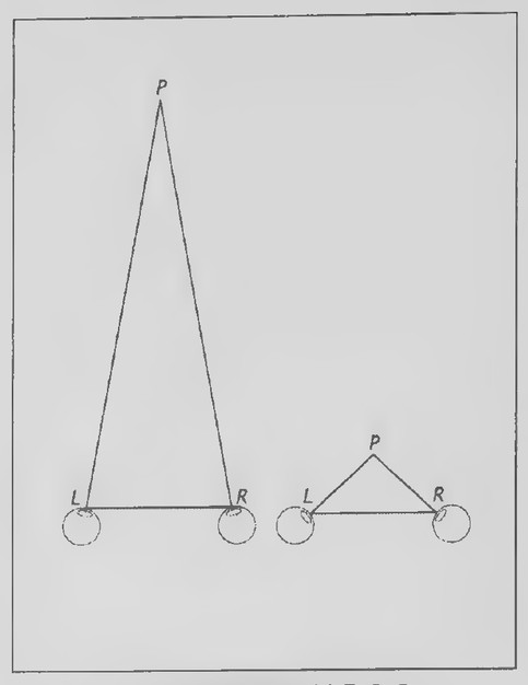Transparency 5-3-2: Convergence when the object is equidistant

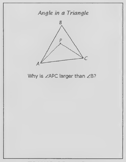Transparency 5-2-3: Angle in a Triangle

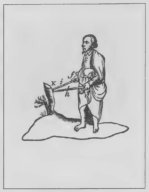Transparency 5-3-1: Blind man judging distance to object

other two figures. You might also ask your students where the UFO would be located when 21 = 22. They may be surprised to find that there is no such location, because 22 is always greater than 21.

The proof of the theorem given in the text implicitly assumes that ray CP lies between rays CA and CD. The authors of the S.M.S.G. Geometry wrote in defense of this assumption:

“It is probably true that no kind of mathematics can be effectively presented in a completely rig orous form to a tenth-grade class. We should not feel guilty about teaching tenth-grade students merely as much as they can learn. The betweenness problem here will probably go unnoticed by most students. It should be called to the attention only of very capable and critical students.”*

Lesson 3: Triangle Side and Angle Inequalities

Lesson Outline

Theorem 13. If two sides of a triangle are unequal, the angles opposite them are unequal in the same order.

Theorem 14. If two angles of a triangle are unequal, the sides opposite them are unequal in the same order.

Transparencies

• 5-3-1 Blind man judging distance to object
• 5-3-2 Convergence when the object is equidistant
• 5-3-3 Convergence when the object is not

equidistant 5-3-4 Triangle drawings (Set I, Exs. 14-22) 5-3-5 Triangle in perspective (Set I, Exs. 23-28) 5-3-6 Not quite equilateral (Set II, Exs. 36-44)

Introduction

The figure on Transparency 5-3-1 shows how a blind man using two sticks might judge the distance to an object. The more that he has to turn the sticks toward each other, the closer the object. The two eyes of a person who is not blind do the same thing. Have your students do the following experiment: Hold a pencil at arm’s length and slowly bring it toward your face while focusing both eyes on it. As your finger comes closer, your eyes turn toward each other, to the extent that you might even appear to be cross-eyed. This turning, called convergence, produces tension in the muscles turning your eyeballs and helps to give your brain information about how close an object is. Try this experiment again, but this time keep the pencil closer to one eye than the other. It is harder to keep focused on your finger this time because one eye has to turn through a bigger angle than the other.

The figures on Transparency 5-3-2 show overhead views of your two eyes converging on the pencil at two different distances. If the pencil is held equidistant from your eyes in each case so that PL=PR, it follows that ∠L = ∠R. Why? (If two sides of a triangle are equal, the angles opposite them are equal.)

The figures on Transparency 5-3-3 also show overhead views of your eyes and the pencil, but here the pencil is held closer to your right eye than your

*School Mathematics Study Group, Geometry —Teacher’s Commentary, Part 1 (Yale University Press, 1961), page 150.

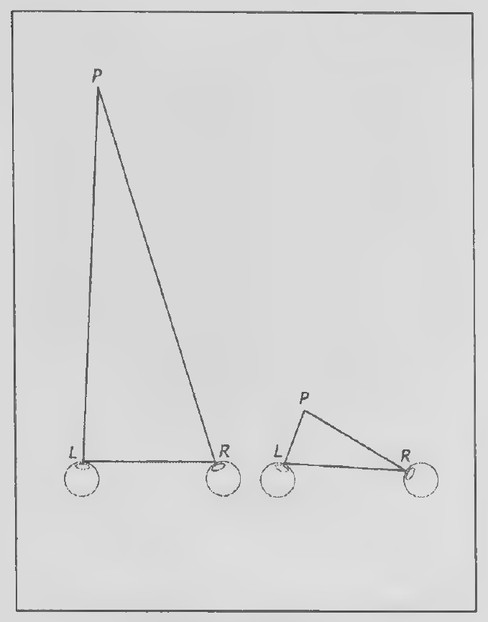Transparency 5-3-3: Convergence when the object is not

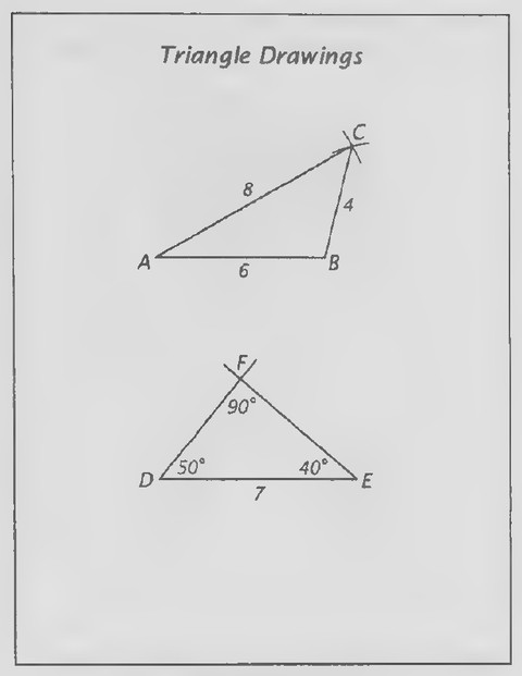Transparency 5-3-4: Triangle drawings (Set I, Exs. 14-22)

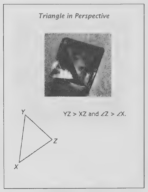Transparency 5-3-5: Triangle in perspective (Set I, Exs. 23-28)

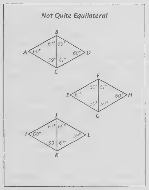Transparency 5-3-6: Not quite equilateral (Set II, Exs. 36-44)

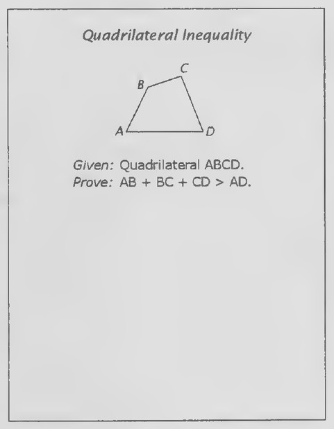Transparency 5-4-1: Quadrilateral inequality (Set II, Ex. 32)

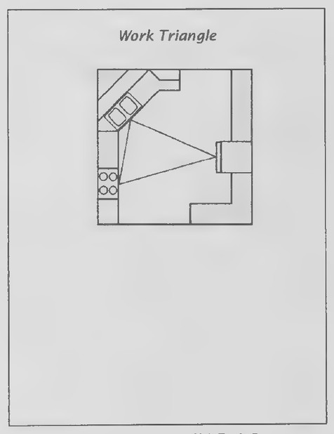Transparency 5-4-2: Work triangle (Set II, Exs. 44-48)

left as it is moved closer. In this case, PL> PR. What has happened to the relative sizes of the angles at L and R² (∠L < ∠R; or, ∠R > ∠L.) Having put this observation into words, your students are now ready for Theorem 13 and its proof.

Lesson 4: The Triangle Inequality Theorem

Lesson Outline

Theorem 15. The Triangle Inequality Theorem. The sum of any two sides of a triangle is greater than the third side.

Transparencies

• 5-4-1 Quadrilateral inequality (Set II, Ex. 32)
• 5-4-2 Work triangle (Set II, Exs. 44-48)

Introduction

Take a stick of uncooked spaghetti, break it into three pieces of approximately equal length, and place them on the overhead projector. Move them together to form the sides of a triangle. Repeat this process with a second stick of spaghetti, but break it into three pieces whose lengths are not quite so close to being equal. Then ask your students if they think that a triangle can always be obtained from the three pieces formed by breaking a stick of spaghetti in this way.

Let a student who realizes that the answer is “no” break a stick into pieces to demonstrate why the answer is correct. This example raises the question of what it is about the lengths of the pieces that determines whether they can or cannot be made into

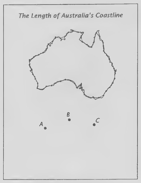Transparency 5-R-2: The length of Australia’s coastline

Transparency 5-R-3: Title page of Spanish mathematics book

Transparency 5-R-1: Satellite photo of Australia

a triangle. Your students are now ready for the Triangle Inequality Theorem and its proof.

Review of Chapter 5

First day

Transparencies

• 5-R-1 Satellite photo of Australia
• 5-R-2 The length of Australia’s coastline
• 5-R-3 Title page of Spanish mathematics book
• 5-R-4 Theorem proof from Spanish mathematics book
• 5-R-5 Gateway arch (Set I, Exs. 5-8)
• 5-R-6 Proof (Set II, Ex. 49)
• 5-R-7 Proof (Set II, Ex. 50)

Introduction

Show Transparency 5-R-1. Do you recognize what is shown in this photograph? (It is a satellite photograph of Australia.*) Two things have been added to the photograph: a grid showing circles of latitude and longitude and the border, or coastline, of Australia, shown in white. Australia is the largest country in the world that is completely surrounded by water. It is easy to measure Australia’s width. It is almost 4,000 kilometers from east to west. To measure the length of Australia’s coastline is another matter. Show Transparency 5-R-2. One way to try to do it is illustrated by the figure at the top. It shows what might happen if a giant walked along the coast. Suppose that each point represents one of the giant’s

footsteps, that the distance between each pair of footsteps is 300 km, and that there are 56 footsteps in all. How far would the giant walk? (56 x 300 km = 16,800 km.) This number, the perimeter of the red polygon, is a rough approximation of the length of the coastline. Now suppose that you walked along the coast. What do you suppose would happen to the apparent length of the coastline if you were to do so? (It would become longer.) This observation suggests something quite strange about the length of Australia’s coastline. What do you suppose it is? (The “length” depends on how you measure it.)

An article in The Australian Geographer? answered the question, “What is the length of the Australian coast?” with “It all depends.” The article went on to state that, when different divider lengths (“distances between footsteps”) are used, the apparent length of the coast steadily increases as the divider length decreases. Steps of 1,000 km suggest a coastline of about 11,000 km; steps of just 1 mm suggest a coastline more than 10 times as long!

The second figure on Transparency 5-R-2 can be used to suggest why the apparent length of the coastline increases as the divider length decreases. Suppose that A, B, and C are three consecutive footsteps along the coast. Why is AB + BC > AC? (The Triangle Inequality Theorem.) Could A,B, and Cbe situated so that AB + BC = AC? (Yes. If A-B-C, then AB + BC = AC.) Could A, B, and C be situated so that AB + BC < AC? (No.)

{What is the length of the Australian coast?” by Robert W. Galloway and Margo E. Bahr (The Australian Geographer, 1979, vol. 3, pp. 244-247).

*Current photographs of Australia, produced by the Japan Meteorological Agency, can be seen on the website: www.bom.gov.au/ weather / satellite /

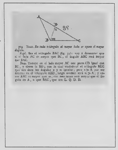Transparency 5-R-4: Theorem proof from Spanish mathematics book

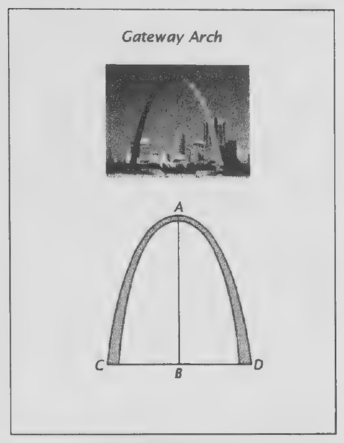Transparency 5-R-5: Gateway arch (Set I, Exs. 5-8)

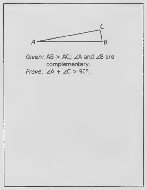Transparency 5-R-6: Proof (Set II, Ex. 49)

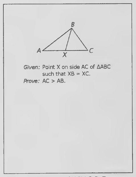Transparency 5-R-7: Proof (Set II, Ex. 50)

Second day

Introduction

Show Transparency 5-R-3. Here is the title page ofa mathematics book of long ago. Can you tell where and when it was published? (Madrid, 1825.) Show Transparency 5-R-4. Here is one of the proofs from this book. Can you translate the theorem into English? (In every triangle, the greater side is opposite the greater angle.) The “given” and “prove” are stated below the theorem. Can you identify them? (Given: In △BAC, AC> BC. Prove: ∠ABC> ∠BAC.)

At this point you might ask your students to draw the figure and write below it our translations of the theorem, “given,” and “prove.” The proof, like the one of page 196 of the text, is Euclid’s. Point out to your students that, although we first encountered this proof in two-column form, it is written here in paragraph form. Although the two-column form is somewhat helpful when a person first learns to write proofs, mathematicians, including Euclid, use paragraph form. Guide your students in listing the main details of the proof as they help you in translating it.

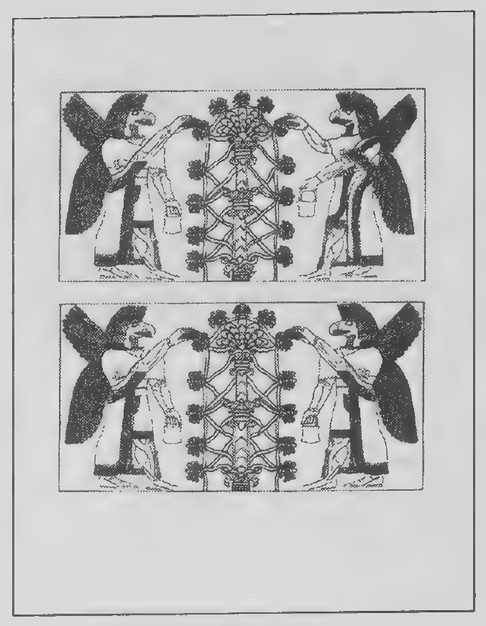Transparency 6-1-1: Assyrian sculpture

Chapter 6: Parallel Lines

Lesson 1: Line Symmetry

Lesson Outline

Terms. Perpendicular bisector, equidistant.

Definition. Two points symmetric with respect to a line.

Theorem 16. Ina plane, two points each equidistant from the endpoints of a line segment determine the perpendicular bisector of the line segment.

Construction 6. To construct a line perpendicular to a given line through a given point.

Transparencies

• 6-1-1 Assyrian sculpture

Introduction

Show the upper figure on Transparency 6-1-1, keeping the lower figure covered. This drawing is of a sculpture created in the seventh century B.C. for the palace in the city of Nimrud (nim-rood) in ancient Assyria (now Iraq). It shows two winged creatures with heads like eagles standing on either side of a tree. They are holding pails and appear to be using sponge-like objects to wash, or possibly fertilize, the tree.

At first glance, the right side of the sculpture might appear to be a mirror image of the left side. Can you see why this is not the case? (One pail is higher than the other. More than that, the arms of the creatures are not mirror images of each other: both creatures are using their right hands to hold the sponges(?) and their left hands to hold the pails.)

Show the lower figure on the transparency. Here the sculpture has been redrawn so that each side is

now the mirror image of the other. The figure now has line symmetry. The two figures are from the book Right Hand, Left Hand by Chris McManus (Harvard University Press, 2002). About them, McManus writes:

Technically, it would have been easier for the artist to draw the bottom picture, and so presumably there were strong reasons… for the additional effort put into drawing the top picture. Not the least of those was probably that the artist knew full well that most people are right-handed, and it was reasonable to presume that eagle-headed spirits would be also. The asymmetry at the heart of the original version of the picture adds to its interest, subtlety and realism, as the eye and the mind flip back and forth between the left and right halves, which are simultaneously similar and different.

Following this introduction, the rest of the lesson can be presented as in the text.

Lesson 2: Proving Lines Parallel

Lesson Outline

Terms: Parallel lines, transversal, corresponding angles, alternate interior angles, interior angles on the same side of a transversal.

Theorem 17. Equal corresponding angles mean that lines are parallel.

Corollary 1. Equal interior angles mean that lines are parallel.

Corollary 2. Supplementary interior angles on the

Transparency 6-2-1: Parallel lines and train tracks

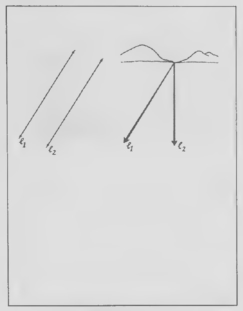Transparency 6-2-2: Parallel lines in perspective

Transparency 6-3-1: Escher’s Waterfall

same side of a transversal mean that lines are

parallel. Corollary 3. In a plane, two lines perpendicular to

a third line are parallel.

Transparencies

• 6-2-1 Parallel lines and train tracks
• 6-2-2 Parallel lines in perspective

Introduction

Show Transparency 6-2-1 and ask your students if the lines are parallel. After someone has explained why he or she thinks that the lines are not parallel, add the overlay. The photograph of the train rails suggests that the lines are parallel after all, but that when they are seen in perspective, they seem to intersect.

Show Transparency 6-2-2. These figures illustrate two different views of parallel lines. The first view shows the lines as seen from overhead and the second view shows them as seen in perspective. Draw a transversal in each figure, label the figures appropriately (see the figures on page 220 of the text), and develop the rest of the lesson as in the text.

Note that the angle relations introduced in this lesson—corresponding angles, alternate interior angles, and interior angles on the same side of the transversal—are not defined, but merely illustrated.

Lesson 3: The Parallel Postulate

Lesson Outline

Construction 7. To construct a line parallel to a given line through a given point.

Postulate 7. The Parallel Postulate. Through a

point not on a line, there is exactly one line

parallel to the given line. Theorem 18. Ina plane, two lines parallel to a third

line are parallel to each other.

Transparencies

• 6-3-1 Escher’s Waterfall

Introduction

To introduce this lesson, you might show Escher’s Waterfall (Transparency 6-3-1). Escher wrote about ihe

Falling water keeps a millwheel in motion and

subsequently flows along a sloping channel be-

tween two towers, zigzagging down to the point

where the waterfall begins again. The miller sim-

ply needs to add a bucketful of water from time

to time, in order to compensate for loss through

evaporation.”

Waterfall was inspired by the Penrose triangle. It appears three times in the picture, which you can show by placing the overlay for Transparency 6-3-1 in the appropriate positions.

Point out that the picture contains several examples of parallel lines and present the rest of the lesson as in the text. It is important to emphasize that “at least one” and “no more than one” are distinct ideas and that proving one does not prove the other. An example such as the following one may be useful. If we wanted to find out how many stu-

*The Graphic Work of M. C. Escher (Meredith Press, 1967; Ballantine Books, 1971).

Transparency 6-5-1: Map: United States, 1858

Transparency 6-4-1: Measuring the height of a cliff

dents at our school might have their birthday today, could we find out if there is at least one by asking everyone in our class? Could we find out if there is no more than one by asking everyone in our class?

Lesson 4: Parallel Lines and Angles

Lesson Outline

Theorem 19. Parallel lines form equal corresponding angles.

Corollary 1. Parallel lines form equal alternate interior angles.

Corollary 2. Parallel lines form supplementary interior angles on the same side of a transversal.

Corollary 3. In a plane, a line perpendicular to one of two parallel lines is also perpendicular to the other.

Transparencies

• 6-4-1 Measuring the height of a cliff

Introduction

The upper figure on Transparency 6-4-1 illustrates a method for indirectly measuring the height of a cliff and is from the first edition of Lancelot Hogben’s Mathematics for the Million (Norton, 1937). In his book Geometry Civilized (Clarendon Press, 1998), J. L. Heilbron describes it:

You want to measure the height of the sheer cliff without climbing it. Put a stick vertically into the sand and draw a circle around its base with a radius equal to the stick’s height. Then wait for a time on a sunny day when the stick’s

shadow just reaches the circle. At that instant, measure the cliff’s shadow, which will equal its height.

The lower figure suggests one way to show why the method works. AB represents the stick and DE represents the cliff. When the stick’s shadow touches the circle at C, we can conclude that AB = BC. Why? (The circle was drawn so that its radius is equal to the stick’s height.) What kind of triangle is △ABC? (Anisosceles right triangle; ∠B is a right angle since the stick was put vertically into the sand.) What can you conclude about the angles at A and C² (∠A = ∠C = 45°.) Since the sun is so far away, it is assumed that the lines represents the rays of light, AC and DF, are parallel. What does this suggest about ∠F² (That it also has a measure of 45°.) Why would it follow from this that the cliff’s shadow is equal to its height? (Assuming that △DEF is also a right triangle, it follows that ∠D = 45° from which we can conclude that the triangle is also isosceles.)

The main assumption in this argument is that parallel lines form equal corresponding angles with a transversal. You might think that we have already proved this as a theorem, but the theorem we have proved is the converse of this. Remember that a statement and its converse do not say the same thing. If a implies b, it does not necessarily follow that b implies a.

Following this introduction, the rest of the lesson can be presented as in the text.

Transparency 6-5-2: Triangulation

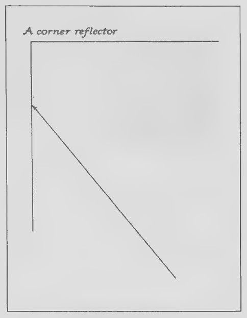Transparency 6-6-1: Acorner reflector

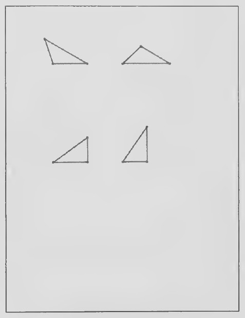Transparency 6-6-2

Lesson 5: The Angles of a Triangle

Lesson Outline

Theorem 20. The Angle Sum Theorem. The sum of the angles of a triangle is 180°.

Corollary 1. If two angles of one triangle are equal to two angles of another triangle, the third angles are equal.

Corollary 2. The acute angles of a right triangle are complementary.

Corollary 3. Each angle of an equilateral triangle is 60°.

Theorem 21. An exterior angle of a triangle is equal to the sum of the remote interior angles.

Transparencies

• 6-5-1 Map: United States, 1858
• 6-5-2 Triangulation

Introduction

The map on Transparency 6-5-1 shows the United States as it appeared in 1858. The strange-looking regions are labeled, from the upper left, Washington, Nebraska, Oregon, Utah, New Mexico, and “Arrizonia.” Oklahoma is labeled “Indian Territory.” This map was copied from a map of railroad surveys undertaken by the U. S. Government to determine the best route from the Mississippi to the Pacific Coast.”

The figure on Transparency 6-5-2 also appears on page 236 of the text and can be used to lead into

the rest of the lesson. In talking about triangulation, it would be interesting to tell your students where the triangulation station mark closest to your school is located. This formation is available from the U. S. Coast and Geodetic Survey.

Lesson 6: AAS and HL Congruence

Lesson Outline

Theorem 22. The AAS Theorem. If two angles and the side opposite one of them in one triangle are equal to the corresponding parts of another triangle, the triangles are congruent.

Theorem 23. The HL Theorem. If the hypotenuse and a leg of one right triangle are equal to the corresponding parts of another right triangle, the triangles are congruent.

Transparencies

• 6-6-1 Acorner reflector
• 6-6-2 . AAS and HL congruence

Introduction

An interesting model that can be used for several purposes consists of two hinged mirrors arranged so that they form a dihedral right angle. Set up such a model in a front corner of the room before class. The model should be approximately at the eye level of your students when they are seated at their desks.

The model is a simple example of a corner reflector: it reflects light back to its source regardless of the direction from which the light comes. This means that all of your students should be able to see their reflections, regardless of where they hap-

*Many interesting maps of the United States are included in The Mapping of America by Seymour I. Schwartz and Ralph E. Ehrenberg (Abrams, 1980).

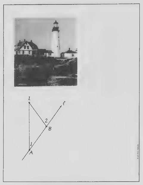Transparency 6-R-1: Doubling the angle on the bow

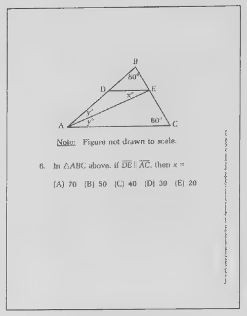Transparency 6-R-2: S.A.T. problem

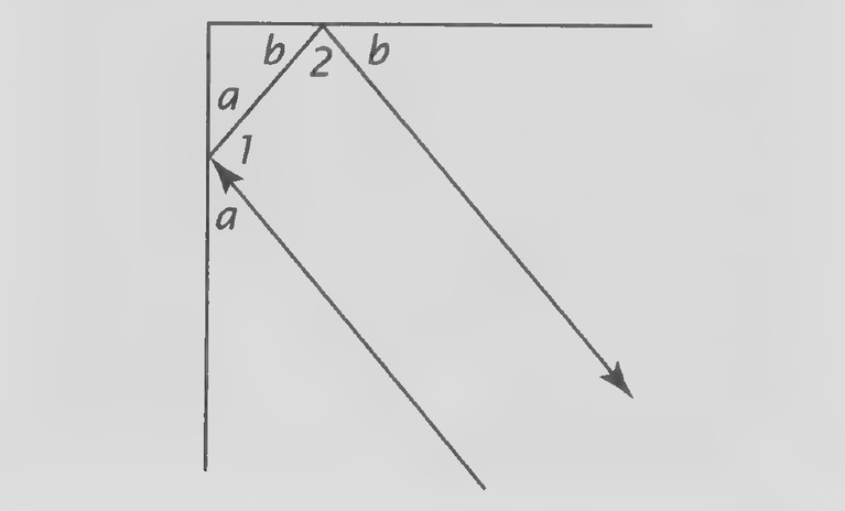Figure on page 340 — A right angle divided by construction lines, with the small angles labelled a, b, 1, and 2

pen to be seated in the room.

Anarray of corner reflectors was left on the surface of the moon at the time of the first landing in 1969. The reflectors make it possible to use laser light to measure the distance from the earth to the moon to within an inch.

Hand out duplicated copies of Transparency 6- 6-1. This figure shows an overhead view of the two mirrors in the corner reflector and a ray of light hitting one of them. Note that the mirrors are perpendicular to each other. The angle at which a ray of light strikes a mirror is equal to the angle at which it is reflected. Your students can discover how the reflector works by using their protractors and rulers to draw the path of the ray of light after it hits the first mirror. The figure that results suggests that the ray of light is reflected back in the same direction from which it came—that is, the incoming and outgoing paths appear to be parallel.

To prove this, label the measures of the angles as shown in the figure below. The proof makes a

good review of several facts from earlier lessons. Guide your students in writing it by observing that a+b=90, 21 =180-2a, and 22 = 180 — 2b, so that

∠1+2Z2 = (180-22) + (180 — 2b)

= 360 - 2a — 2b

= 360-2(a +b)

= 360 - 2(90)

= 180. Because we have shown that 21 and 22 are supplementary, it follows that /, and I, are parallel.

I suggest providing your students with duplicated copies of Transparency 6-6-2 for use in taking notes on the proofs of the AAS and HL congruence theorems.

Review of Chapter 6

Transparencies

• 6-R-1 Doubling the angle on the bow
• 6-R-2 S.A.T. problem

First day

Introduction

One of the seven wonders of the ancient world was a lighthouse at Alexandria in Egypt. Built at about the time of Euclid, it guided ships until as late as the twelfth century. Today more than 10,000 lighthouses mark the shorelines of the world’s continents for ships traveling at night.

An example of how the navigator of a ship uses geometry to determine how far the ship is from a lighthouse sighted on the shore is illustrated on Transparency 6-R-1. This procedure is called “doubling the angle on the bow.” Suppose that the ship

is moving along line / when a lighthouse at point L is sighted. As the ship travels along the line, the angle between its course and the line of sight to the lighthouse gets larger and larger. If the navigator measures this angle when the ship is at A and then waits until the ship has moved to a point where the angle has doubled, point B in the figure, the navigator can conclude that the distance from the ship to the lighthouse is equal to the distance the ship has traveled in going from A to B. In other words, if 22 =2/1, then LB = AB.

Give your students time to try to write a proof of this procedure, taking as “given” that 22 = 2/1 and that 22 is an exterior angle of △ABL.

Proof.

1. 22 =221 and 22 is an exterior angle of

△ABL. (Given.)

2. ∠2= 21+ ∠L. (An exterior angle of a

triangle is equal to the sum of the remote

interior angles.)

. 221 = 21+ ∠L. (Substitution.)

. ∠1 = ∠L. (Subtraction.)

O ® O1. LB=AB. (If two angles of a triangle are

equal, the sides opposite them are equal.)

Second day

Introduction

The S.A.T. problem on Transparency 6-R-2 provides further review of ideas in Chapter 6.

Transparency 7-2-2: Acrossword puzzle pattern

Transparency 7-1-1: Photograph of mud cracks

Transparency 7-2-1: The first crossword puzzle

Chapter 7: Quadrilaterals

Lesson 1: Quadrilaterals

Lesson Outline

Terms: Convex polygon, concave polygon, diagonal of a polygon, rectangle.

Theorem 24. The sum of the angles of a quadrilateral is 360°.

Corollary. A quadrilateral is equiangular iff it is a rectangle.

Transparencies

• 7-1-1 Photograph of mud cracks

Introduction

Show Transparency 7-1-1 and let your students guess what the photograph is of. It shows cracks in dried mud and is taken from a fascinating book that every mathematics teacher should own: Mathematical Snapshots by Hugo Steinhaus (Oxford University Press, 1969).

Can you guess which cracks occurred first? (The longest ones.) It is interesting to notice that almost all of the cracks meet at right angles. (There is a physical explanation for this in terms of the laws of mechanics.) Most of the figures formed by the cracks have four sides; they are examples of quadrilaterals, the subject of the next chapter of the course.

(Add the Overlay for Transparency 7-1-1.) Certain types of quadrilaterals are given specific names; some examples are shown here. How many of them

can you identify? (1. square; 2. rectangle; 3. parallelogram; 4. trapezoid.)

Lesson 2: Parallelograms and Point Symmetry

Lesson Outline

Terms: Parallelogram, point symmetry.

Theorem 25. The opposite sides and angles of a parallelogram are equal.

Theorem 26. The diagonals of a parallelogram bisect each other.

Transparencies

• 7-2-1 The first crossword puzzle
• 7-2-2 Acrossword puzzle pattern

Introduction

The first crossword puzzle was published in the New York World on December 21, 1913 and is shown on Transparency 7-2-1. Unlike current crossword puzzles, it was diamond shaped and did not contain any black squares. Today, crossword puzzles appear daily in almost every American newspaper. They are almost always square and the black squares in them are usually arranged in symmetric patterns.

The arrangement shown on Transparency 7-2-2 is a typical example. The pattern does not have line symmetry because there is no way to fold it so that the two halves coincide. It has a different kind of symmetry. Can you describe what it is? (The pat-

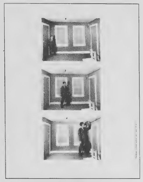Transparency 7-3-1: The Ames room

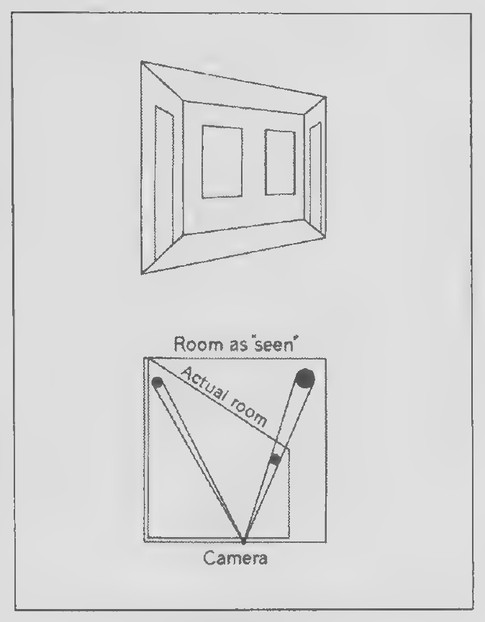Transparency 7-3-2: The Ames room explained

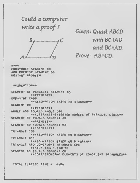Transparency 7-4-1: Could a computer write a proof?, 1

tern would look the same if it were turned upside down.) A figure having this property is said to possess point symmetry. Mark the point that is the center of the pattern and show examples of pairs of points in the pattern that are symmetric with respect to this point. What relation does this point have to the line segments connecting such pairs of points? (It is their midpoint.)

The grid of a crossword puzzle contains squares and rectangles, both of which also possess point symmetry. It also contains parallelograms; squares and rectangles are also called parallelograms because their opposite sides are parallel. Following from this introduction, the rest of the lesson can be developed as in the text.

Lesson 3: More on Parallelograms

Lesson Outline

Theorem 27. A quadrilateral is a parallelogram if its opposite sides are equal.

Theorem 28. A quadrilateral is a parallelogram if its opposite angles are equal.

Theorem 29. A quadrilateral is a parallelogram if two opposite sides are both parallel and equal.

Theorem 30. A quadrilateral is a parallelogram if its diagonals bisect each other.

Transparencies

• 7-3-1 The Ames room
• 7-3-2 The Ames room explained

Introduction

Transparencies 7-3-1 and 7-3-2 can be used to introduce the new lesson as in the text. The Ames room

was invented by the American psychologist Adelbert Ames. Some interesting experiments with an Ames room are described in the article “Visual Perception and Personality” by Warren J. Wittreich in the April 1959 issue of Scientific American (pages 56-60).

Lesson 4: Rectangles, Rhombuses, and Squares

Lesson Outline

Terms: Square, rhombus.

Theorem 31. All rectangles are parallelograms.

Theorem 32. All rhombuses are parallelograms.

Theorem 33. The diagonals of a rectangle are equal.

Theorem 34. The diagonals of arhombus are perpendicular.

Transparencies

• 7-4-1 Could a computer write a proof?, 1
• 7-4-2 Could a computer write a proof? (2)

Introduction

Not long after the invention of the computer, an experiment was conducted at the IBM Research Laboratory to see if a computer could be programmed to write geometric proofs. A number of basic postulates and theorems, along with the methods of deductive reasoning, were stored in the memory of an IBM 704 computer and then it was given some exercises to prove. One of them is similar to a theorem in yesterday’s lesson. Show Transparency 7-4-1. The problem was to show that, if two sides of a quadrilateral are both parallel and equal, then the other two sides are equal. This is what the computer did. Show Transparency 7-4-2. Your stu-

Transparency 7-5-1: Greek parallelogram and trapezoids

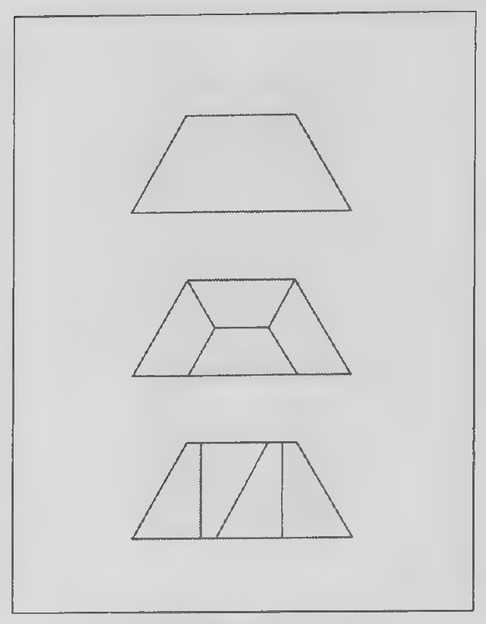Transparency 7-5-2: Congruence puzzle (Set III)

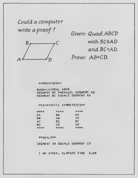Transparency 7-4-2: Could a computer

dents should recognize the “premises” and “goals” as the “given” and “prove.” The “syntactic symmetries” are a list of point relations that had to be included in the program because the computer could not see the figure.

After the computer had “thought” about the problem for 88 seconds, it reported that it was stuck (some of my students exhibit about the same amount of persistence, I am afraid). The computer was stuck because it did not know very much about quadrilaterals. To help out the computer, the person running it added a diagonal to the figure to form some triangles. After a few more minutes, the computer printed out the proof given. As you read it to the class, point out that we would take some of the steps for granted.

If the computer had been programmed with the theorems of yesterday’s lesson, it might have come up with a much shorter proof. Can you think of what it is? (The quadrilateral is a parallelogram because two opposite sides are both parallel and equal. The opposite sides of a parallelogram are equal.)

Your students will be interested to know that in 1976, two mathematicians at the University of Illinois used a computer to finally prove a theorem that people had been trying to prove since its discovery in 1852.* Unfortunately, the proof is so long that it would be impossible for a human being to read it. It took 1,200 hours of computer time to write the

proof and it would take more than a lifetime to read it!

Lesson 5: Trapezoids

Lesson Outline

Terms: Trapezoid, bases, legs, base angles, isosceles trapezoid.

Theorem 35. The base angles of an isosceles trapezoid are equal.

Theorem 36. The diagonals of an isosceles trapezoid are equal.

Transparencies

• 7-5-1 Greek parallelogram and trapezoids
• 7-5-2 Congruence puzzle (Set III)

Introduction

Hand out duplicated copies of Transparency 7-5-1. It is interesting to realize that some of the words that we use in geometry would sound familiar to Euclid, even though he lived in Egypt more than two thousand years ago. The figures and words are from a geometry book written in Greek.

Have your students identify the figures and print their English names in capital letters below the Greek names. The Greek word “parallelogrammon” is derived from words meaning “bounded by parallel lines.” “Trapezion’ is related to trapezoid and the Greek word “isosceles” means “having equal legs.”

Transparency 7-5-2 is for use in discussing the Set III exercise of Lesson 5. The figure in the center was originally thought to be the only solution to

*The theorem is the four-color map theorem referred to on page 6 of the text. An interesting book on this subject is Four Colors Suffice: How the Map Problem was Solved by Robin Wilson (Princeton University Press, 2002).

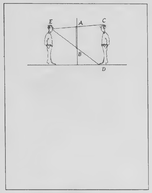Transparency 7-6-1: The mirror on the wall

this puzzle but Andrew Miller, the high school student of Richard Brady in Washington, D.C. mentioned in the text, discovered the solution pictured at the bottom. This solution was sufficiently surprising that it was reported in Scientific American (Martin Gardner’s “Mathematical Games,” February 1979).

Lesson 6: The Midsegment Theorem

Lesson Outline

Terms: Midsegment

Theorem 37. The Midsegment Theorem. A midsegment of a triangle is parallel to the third side and half as long.

Transparencies

• 7-6-1 The mirror on the wall

Introduction

If possible, place a large mirror on one of the walls of your room before class. Be sure that the mirror is vertical.

You have all looked at reflections of yourselves in large wall mirrors. How do you suppose your distance from the mirror affects the amount of yourself that you can see? (Because the farther you are from the mirror, the farther your reflection seems to be behind it, many people assume that you can see more of yourself as you move away from the mirror. Some people, realizing that, as you back away from a mirror you see less and less of the surrounding room reflected in it, think that you see less of yourself as well. Actually, your distance from the mirror makes no difference. The amount of your-

self that you can see is controlled solely by the length of the mirror and not by how far away from it you happen to be standing. A student who walks from the back of the room toward the mirror at the front while looking at his or her reflection can confirm this.)

To see why this is so, look at this diagram (Transparency 7-6-1). The vertical segment in the center represents a side view of a wall and AB represents a mirror on it. The mirror is just long enough so that the person standing on the left can see his entire image on the right. (Add Overlay A.) If the person moves away from the mirror, so does his image. Notice, however, that his lines of sight to the reflections of the top of his head and bottom of his feet still pass through points A and B. (Replace Overlay Awith Overlay B.) This figure shows what happens if the person moves toward the mirror instead. Again, his lines of sight pass through points A and B. (Remove Overlay B.) How long do you think the mirror would need to be for the person to see his entire image if he is six feet tall? In other words, if CD = 6, how long do you think AB is? It is not difficult to prove that A and B are the midpoints of sides EC and ED in △ECD. We will call a segment that joins the midpoints of two sides of a triangle a midsegment of the triangle, and we will prove that such a segment is always parallel to the third side of the triangle and exactly half as long. The rest of the new lesson can be developed as in the text.

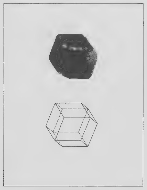Transparency 7-R-1

Transparency 7-R-2: Square illusion

WORKSHEET FOR 7-R

Review of Chapter 7

Transparencies

• 7-R-1 _ Garnet crystal and polyhedron
• 7-R-2 Square illusion
• 7-R-3 Quadrilateral quiz Square illusion (worksheet)

First day

Introduction

Transparency 7-R-1 contains a photograph of a crystal of garnet and a diagram of its structure.* Every edge of the crystal has the same length, and so its faces are equilateral. What kind of faces does the crystal have? (Rhombuses.) What other names for them can you think of? (Parallelograms, quadrilaterals, polygons.)

As a review of the various quadrilaterals studied in this chapter, you might direct your students in making an outline such as the one shown at the right.

Second day

Introduction

Show Transparency 7-R-2 with the overlay in place and ask your students what kind of quadrilateral they think is pictured. (Square and rectangle are popular guesses.) Then hand out duplicated copies of Worksheet for Chapter 7 Review and give everyone a chance to measure the sides of the quadrilat-

eral with their rulers. After they have discovered that the left and right sides are not equal, remove the overlay from the transparency to reveal the quadrilateral as an isosceles trapezoid. This is quite a remarkable optical illusion!

Next, hand out duplicated copies of Transparency 7-R-3 and tell your students that, although these figures look like the quadrilateral in the optical illusion, they are not to make any assumptions about the figures other than what you tell them. The

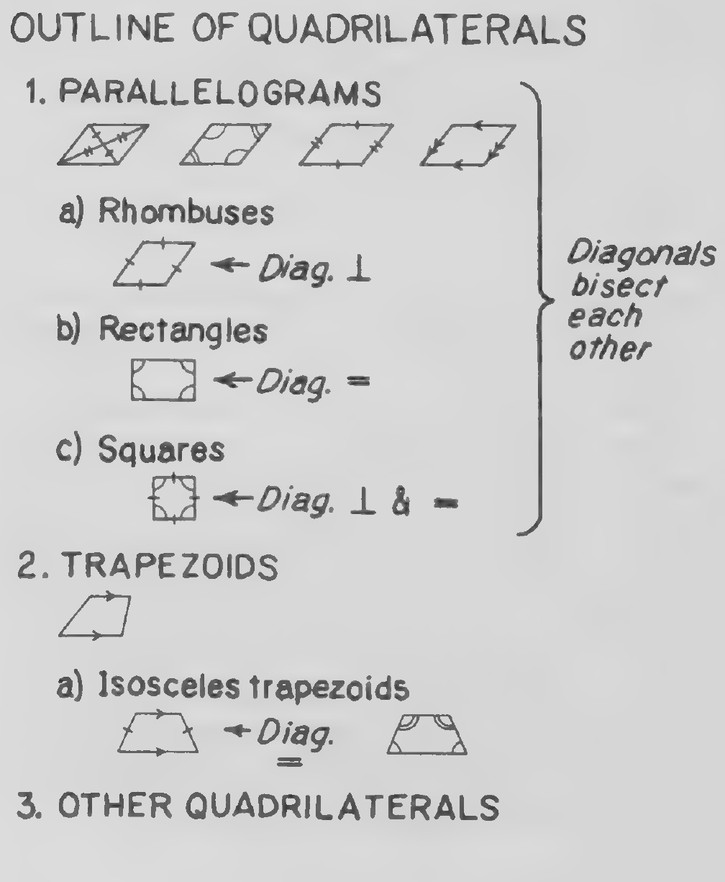Worksheet: outline of quadrilaterals

The outline classifies quadrilaterals: parallelograms (a. rhombuses, b. rectangles, c. squares — the diagonals of all three bisect each other; in rhombuses they are perpendicular, in rectangles equal, and in squares both), trapezoids (a. isosceles trapezoids), and other quadrilaterals.

*This solid, called a rhombic dodecahedron, has 12 identical faces: each face is a rhombus having acute angles of 70°32’. An interested student might enjoy making a model of it for you to use.

Transparency 7-R-3: Quadrilateral quiz

figure at the upper left is for use as an example. Use arrowheads to mark the top and bottom parallel and explain that the problem, if it is possible, is to identify the type of quadrilateral as specifically as they can. If it is not possible, they are to answer with a question mark. In the case of the example, we do not know anything about the other two sides. The figure could be a parallelogram or a trapezoid, and so the correct answer is a question mark.

Before beginning the quiz, you might mention that the questions vary in difficulty from very easy to very tricky. I tell my students that anyone who is able to answer all twelve questions correctly deserves an A on the chapter. Ask all twelve questions before checking the answers.

What you draw

on the figure The answer

1. Mark the vertical sides Parallelogram

parallel and equal.

2. Mark all four angles Rectangle

equal.

3. Mark both pairs of Parallelogram

opposite sides parallel.

4. Mark the vertical sides?

equal.

5. Mark all four sides Rhombus

equal.

6. Mark both pairs of Parallelogram

opposite angles equal.

7. Mark all four sides Square

equal and all four

angles equal.

8. Mark the top and 2

bottom parallel and the

vertical sides equal.

9. Draw the diagonals Parallelogram

and indicate that they

bisect each other. 10. Mark both pairs of Parallelogram

opposite sides equal. 11. Mark one pairofop-?

posite angles equal. 12. Draw the diagonals?

and mark them

perpendicular.

The last question is particularly treacherous because it is so easy for students who know that the diagonals of a rhombus are perpendicular to make the converse error.

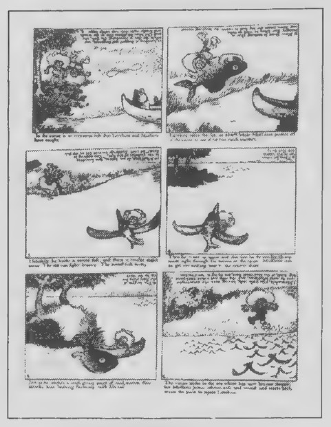Transparency 8-1-2: Upside-downs cartoon strip

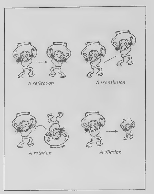Transparency 8-1-3: More transformations

Transparency 8-1-1: Upside-downs cartoon

Chapter 8: Transformations

Lesson 1: Transformations

Lesson Outline

Terms: Transformation, translation, reflection, rotation, dilation, isometry.

Transparencies

• 8-1-1 Upside-downs cartoon
• 8-1-2 Upside-downs cartoon strip
• 8-1-3 More transformations

Introduction

One of the earliest comic strips to appear in a newspaper was also one of the most remarkable. Its title was “The Upside-Downs of Little Lady Lovekins and Old Man Muffaroo” and it was published in the New York Herald from 1903 to 1905. The two characters of the cartoon are shown on Transparency 8-1-1. They were drawn so that each character became the other when turned upside down.

One of the comic strips in which these characters appeared is on Transparency 8-1-2. After reading it to your class, point out the amazing aspect of the strip. Not only does each panel make sense upside down, but the story also makes sense even though the first six panels of the strip become the last six panels in reverse order. The artist, Gustave Verbeek, drew a comic strip like this every week for a total of 64 weeks! His work is surely the most amazing application that the rotation transformation has ever had to the field of storytelling and art.

Transparency 8-1-3 can be used to develop the rest of the lesson as in the text.

Lesson 2: Reflections

Lesson Outline

Terms: Reflection of a point through a line, composite, translation, rotation, magnitude.

Construction 8. To reflect a point through a line.

Transparencies

• 8-2-1 Reflection in a lake

Introduction

Show Transparency 8-2-1, which is a photograph of Lake Mathieson in New Zealand. There is something peculiar about this picture. Can you guess what it is? The photograph is upside down. We were fooled by the almost perfect reflection of the landscape and sky in the water into mistaking their images for them. (Turn the picture rightside up.) The edge of the lake divides the picture into two parts in which most of the points above the edge have image points below it. (Draw a line along the lake’s edge and mark several such pairs of points on the picture at various distances from the line. Include one point on the line.) Your students should note that the reflection line is the perpendicular bisector of the segments joining the points to their image points. On the basis of these observations, we will build a “mathematical model” of reflection.

Transparency 8-2-1: Reflection in a lake

Transparency 8-3-1: “Separate checks, please”.

Transparency 8-3-2: Alanine stereoisomers

Develop the rest of the lesson, including the method for locating the reflection of a point through a line by means of straightedge and compass, as in the text.

Lesson 3: lsometries and Congruence

Lesson Outline

Terms: Congruence, glide reflection, mirror image.

Transparencies

• 8-3-1 “Separate checks, please”.
• 8-3-2 Alanine stereoisomers

Introduction

From what the fellow in the cartoon on Transparency 8-3-1 is saying to the waiter, it is apparent that he does not realize that the man sitting at the next table is his own reflection. Perhaps he doesn’t want to pay for all eight drinks because he was irritated by observing that the other person copied everything he did during the meal!

Here is something interesting to think about. Suppose that one of the glasses in front of the man were still full; its image in the mirror, then, would also be full. If it were possible for the man to reach through the mirror and take a drink from the reflected glass, would it taste the same as the drink in the glass in front of him? The answer to this question is “probably not”!*

The figures on Transparency 8-3-2 illustrate two molecules, each of which is the mirror image of the other. Molecules such as these are called stereoisomers. In his book The Architecture of Molecules (W. H. Freeman and Company, 1964), Linus Pauling states that only “left-handed” molecules of the amino acid alanine occur in the proteins of living organisms. The other amino acids in proteins also are left-handed. Some of the right-handed amino acids cannot serve as nutrients and they may, in fact, be poisonous.

Lesson 4: Transformations and Symmetry

Lesson Outline

Terms: Rotation symmetry, reflection (line) symmetry, translation symmetry.

Transparencies

• 8-4-1 Upside-down names by Scott Kim
• 8-4-2 Inversions by Scott Kim
• 8-4-3 Symmetry examples

Introduction

The names of Transparency 8-4-1 are from a clever book by Scott Kim, who might be called the “Maurits Escher of calligraphy.” Mr. Kim letters words and phrases in amazingly symmetrical pat-

passage from W. H. Auden’s poem The Age of Anxiety in which a right-handed man sitting in a bar and observing his reflection in a mirror says:

My deuce, my double, my dear image,… What flavor has

That liquor you lift with your left hand…?

*Some of your students would enjoy reading a fascinating book by Martin Gardner on this subject: The Ambidextrous Universe: Mirror Asymmetry and Time-Reversed Worlds, Second Edition (Scribners, 1979). In this book, Gardner quotes a

Transparency 8-4-1: Upside-down names by Scott Kim

Transparency 8-4-2: Inversions by Scott Kim

Transparency 8-4-3: Symmetry examples

Transparency 8-R-1: U.S. currency

Transparency 8-R-2: Cutting corners

Transparency 8-R-3: Hall of mirrors photograph

terns. Rotating the transparency 180° reveals that each name looks the same upside down. The names have been lettered so that they have rotation symmetry. A figure has rotation symmetry with respect to a point if it coincides with its rotation image about the point. The figure on Transparency 8-4-2 does not have rotation symmetry, but it is remarkable in that it is the name of Scott Kim’s book, Inversions, and, upside down, becomes Scott Kim’s name.

Show the picture of a butterfly on Transparency 8-4-3, keeping the figure below covered, as an example of reflection symmetry. A second copy of the paper-windmill figure to use with the figure on Transparency 8-4-3 is helpful to show that it does not have reflection symmetry but that it does have rotation symmetry. Show how the windmill can be

rotated 90°, 180°, or 270° to coincide with itself.

Review of Chapter 8

Transparencies

• 8-R-1 U.S. currency
• 8-R-2 Cutting corners
• 8-R-3 Hall of mirrors photograph
• 8-R-4 Hall of mirrors diagram
• 8-R-5 Big Dipper

First day

Introduction

Show Transparency 8-R-1. A bill was once submitted to Congress proposing that U.S. currency be printed in a way that enables a person who is blind to determine the denomination of each note. It was

Transparency 8-R-4: Hall of mirrors diagram

Transparency 8-R-5: Big Dipper

suggested that some of the corners of the notes be trimmed so that the values of the notes could be figured out by their shapes.

The seven denominations of bills currently in circulation are shown on the transparency. How many ways are there to cut (or not cut) the corners of a rectangle so that each shape is different? Assume that the cuts are angled at 45° and identical in size.

Hand out duplicated copies of Transparency 8-R-2 and give your students some time to try to discover all of the possibilities. Remind them that a blind person feeling a bill does not know what position the bill is in; considerations of symmetry are important in finding ways that are really different.

It is somewhat of a coincidence that there happen to be exactly seven different ways to cut (or not cut) the corners. They are:

No corners.

. One corner.

Two adjacent corners along a short edge.

. Two adjacent corners along a long edge.

. Two opposite corners.

Three corners.

PWN QO N. Four corners.

After the solutions have been found, it is interesting to think about how each particular denomination of bill should be cut. Which bill, for example, should have no corners cut and which should have all four corners cut? (The corners of the bills should be cut so that a person cannot deceive someone who is blind by cutting off additional corners to make them seem more valuable. Therefore, the $1 bill

should have all four of its corners cut. The $2 bill should have three corners cut; the $5, $10, and $20 bills should have two corners cut; the $50 bill should have one corner cut; and the $100 bill should have no corners cut.)

Second day

Introduction

There is an elaborate maze of mirrors in Lucerne, Switzerland, that was originally built for the Swiss National Exhibition of 1896. A photograph showing part of the maze appeared on the cover of the June 1986 issue of Scientific American (Transparency 8-R-3). The floor plan of the maze, shown on Transparency 8-R-4, consists of an array of equilateral triangles. Mirror walls stand on one or two sides of most of these triangles and several scenes, shown on the floor plan, are inside the maze.

Hand out duplicated copies of Transparency 8-R-4 and explain that, if you stood at the entrance of the maze, you would see what looks like a long hallway. The problem is to use reflections to figure out what you would see at the end of the hallway. Help your students in getting started by drawing a line from the center of the entrance to represent a ray of light and showing its first two reflections from the walls. It may be helpful to think of the path as that of a ball rolled into the maze and bouncing around until it hits a surface that is not a mirror. A person standing at the entrance to the maze would see the scene enclosed in the upper triangle.

Asecond problem might be to figure out to what point in the maze you would have to walk in order to see the triangle filled with flowers. (You would

have to walk into the triangle adjacent to the first scene.)

Students who have enjoyed solving these reflection problems will find “The Amateur Scientist” column in the June 1986 issue of Scientific American very interesting. The column, by Jearl Walker, includes another color photograph of the Hall of Mirrors in Lucerne and suggests a variety of experiments to perform to learn more about mirror mazes.

An interesting class exercise for additional review is illustrated on Transparency 8-R-5, which should be duplicated and given to your students. Explain that during the night, the stars of the Big Dipper appear to rotate counterclockwise about Polaris, the north star. In the figure, two positions of the Big Dipper are shown. The first problem is to find Polaris, the center of the rotation. The second problem is to find the magnitude of the rotation. (75°.) The final problem is to estimate the length of time that it takes the Big Dipper to move in the sky from one of these positions to the other. (Five hours.)

Transparency 9-1-1: Map: Kansas and surrounding states

Transparency 9-1-2: Map: United States

Chapter 9: Area

Lesson 1: Area

Lesson Outline

Terms: Polygonal region.

Postulate 8. The Area Postulate. Every polygonal region has a positive number called its area such that (1) congruent triangles have equal areas and (2) the area of a polygonal region is equal to the sum of the areas of its nonoverlapping parts.

Transparencies

• 9-1-1 Map: Kansas and surrounding states
• 9-1-2 Map: United States

Introduction

Show Transparency 9-1-1. The earth’s present (2003) population is about 6,300,000,000 people.* Suppose that everyone moved to the state of Kansas: how crowded would it be? (Add the overlay to the transparency.) At the center of the United States, Kansas has an area of about 82,000 square miles. If all 6,300,000,000 people lived in Kansas, what would be the average number of people per square mile? (Approximately 77,000.)

Let’s see how this figure compares with the “population density” of our school. (Give your class the approximate area of your campus as a fraction of a square mile and the number of people on it so that they can find out. For example, the campus of the school at which I teach has an area of about 1/20 square mile and about 3,600 people on it during the school day; hence its “population density” is about 72,000 people per square mile.) According to the Guinness Book of World Records, the most densely populated region in the world is in a section of Hong Kong, with more than 650,000 people per square mile!

Point out that in each of our calculations, we used a number called the area of the region. The idea of “area” is a very fundamental one in geometry and it is the subject of the next chapter of the course.

Show the map of the continental United States on Transparency 9-1-2. The fifty states vary in size from about 591,000 square miles (Alaska) to slightly more than 1,200 square miles (Rhode Island). Note that the areas of states such as Wyoming, Colorado, and Utah are relatively simple to determine, whereas the area of a state such as Florida is not as easily found. Have your students draw a figure representing Utah and use it to introduce the idea of a polygonal region and the Area Postulate.

*Give the appropriate figure for the current year.

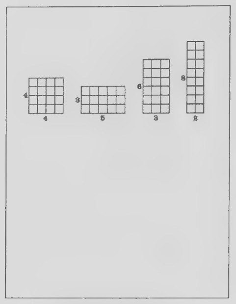Transparency 9-2-1: National Assessment problem on area

Transparency 9-2-2: World’s longest mural

Lesson 2: Squares and Rectangles

Lesson Outline

Terms: Dimensions of a rectangle: base and altitude.

Postulate 9. The area of a rectangle is the product of its base and altitude.

Corollary. The area of a square is the square of its side.

Transparencies

• 9-2-1 National Assessment problem on area
• 9-2-2 World’s longest mural

Introduction

The figures on Transparency 9-2-1 once appeared in a question on a mathematics test (The National Assessment of Educational Progress) given to nineyear-olds all over the United States. The question was: Which rectangle has the same area as the 4 x 4 square?

After a student gives the correct answer, ask how he or she would explain it to a student who missed it. Only 44% of the students chose the correct answer. Almost as many chose the 3 x 5 rectangle. Can you explain why? (Your students may have a variety of answers for this.) After discussing the difference between perimeter and area, add the overlay to the transparency. We measure area in terms of square units. From these examples, it would seem that the area of a rectangle can always be found by dividing it into these square units and counting them. A shortcut for finding the number of squares would be to multiply the lengths of the “base” and “altitude.”

Develop the rest of the lesson as in the text, emphasizing that, because the dimensions of a rectangle are not always integers, we assume that the shortcut gives the area for every rectangle.

The following exercise is appropriate for the conclusion of this lesson. The longest mural in the world is located next to the school at which I teach (Grant High School, Van Nuys, California). It is called “The Great Wall of Los Angeles”; the photograph on Transparency 9-2-2 shows part of it as well as part of our campus. The mural is 2,000 feet long and 13.5 feet high. A gallon of the paint used covered an area of 150 square feet. On the basis of these figures, how many gallons of paint were needed to produce the mural? (180.)

Transparency 9-2-3 is for use in demonstrating the solution of the Set III exercise. More information about dividing rectangles into squares all having different areas can be found in The Second Scientific American Book of Mathematical Puzzles and Diversions by Martin Gardner (Simon & Schuster, 1961), pages 186-209 and Ingenuity in Mathematics by Ross Honsberger, in the New Mathematical Library (M.A.A., 1970), pages 46-60.

Transparency 9-3-1: A land bonanza in the Klondike

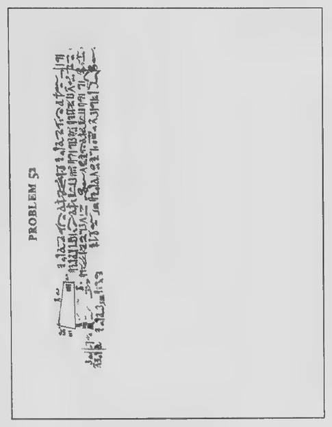Transparency 9-4-1: Problem 52 from the Rhind Papyrus

Lesson 3: Triangles

Lesson Outline

Terms: Base and altitude of a triangle.

Theorem 38. The area of a right triangle is half the product of its legs.

Theorem 39. The area of a triangle is half the product of any base and corresponding altitude.

Corollary. Triangles with equal bases and equal altitudes have equal areas.

Transparencies

• 9-3-1 A land bonanza in the Klondike

Introduction

Show Transparency 9-3-1. In the 1950s, the Quaker Oats Company sponsored a radio program called “Sergeant Preston of the Yukon.” They once made an offer on their program to sell anyone who sent in 25¢ and a coupon from a box of their cereal some land in the Klondike. For your money, you got a deed to your new property and a small bag of dirt from the general vicinity. Of course, you couldn’t expect a very big lot for only 25¢ and, in fact, each lot was only one square inch in area!

At this rate, how much was one acre of the land being sold for?* One acre is equal to 43,560 square feet. (One acre would have sold for $1,568,160!) The company didn’t make any significant profit, however, because most of the 25¢ went toward the costs

of preparing and mailing the deeds and samples of dirt.

Lesson 4: Parallelograms and Trapezoids

Lesson Outline

Terms: Altitude of a quadrilateral.

Theorem 40. The area of a parallelogram is the product of any base and corresponding altitude.

Theorem 41. The area of a trapezoid is half the product of its altitude and the sum of its bases.

Transparencies

• 9-4-1 Problem 52 from the Rhind Papyrus

Introduction

In 1858, a tourist named Rhind bought an old scroll in a shop in Egypt. The scroll, which is now in the British Museum, turned out to have been written in about 1650B.C. Now called the Rhind Mathematical Papyrus, this scroll is the major source of our knowledge of early Egyptian mathematics.’ It was copied by the scribe Ahmes from earlier writings and contains 87 problems in arithmetic and geometry.

Problem 52 of the Papyrus is shown on Transparency 9-4-1. The problem says:

A cut-off triangle of land is 20 khet on one side, 6 khet on its base, and 4 khet on its cut-off line. What

*This is adapted from a problem in The Lore of Large Numbers by Philip J. Davis, in the New Mathematical Library (M.A.A., 1961).

tThe translation of The Rhind Mathematical Papyrus by Arnold Buffum Chace was published by the N.C.T.M. as volume 8 of the “Classics in Mathematics Education” series.

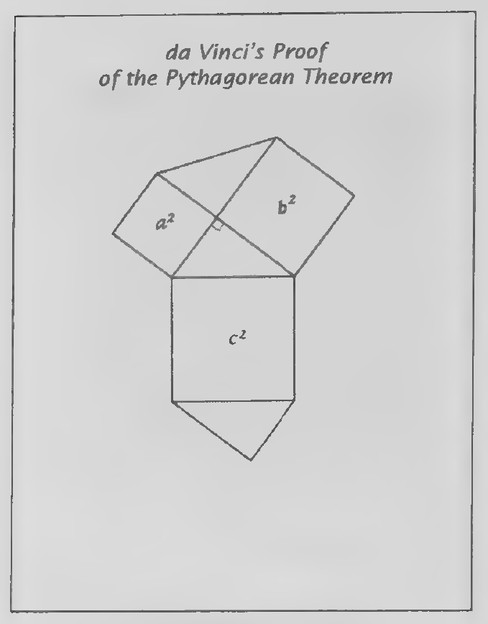Transparency 9-5-1: Da Vinci’s proof of the Pythagorean

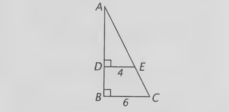Figure on page 356 — Leonardo da Vinci’s proof diagram: triangle ABC with the perpendiculars and auxiliary segments labelled

is its area? [A khet is equal to 100 cubits, which is roughly 150 feet.]

Although the statement of this problem is rather vague and the figure illustrating it is not accurately drawn, the way in which it is solved makes clear that the problem is about a trapezoid cut off froma right triangle. Have your students draw the following figure to illustrate it.

Although we a formula for the area of a trapezoid, we can find the area of this trapezoid by dividing it into a rectangle and a right triangle. Give your students time to do this before discussing the solution. Drawing a perpendicular from E to BC, we have a rectangle with area 80 and a right triangle with area 20; the area of the trapezoid is 100 square khets.

Following this introduction, the formulas for the areas of a parallelogram and a trapezoid can be derived. Now the Egyptian problem can be reconsidered in terms of the trapezoid area theorem.

Lesson 5: The Pythagorean Theorem

Lesson Outline

Theorem 42. The Pythagorean Theorem. The square of the hypotenuse of a right triangle is equal to the sum of the squares of its legs.

Theorem 43. Converse of the Pythagorean Theorem. If the square of one side of a triangle is equal to the sum of the squares of the other two sides, the triangle is a right triangle.

Transparencies

• 9-5-1 Da Vinci’s proof of the Pythagorean Theorem
• 9-5-2 Converse of the Pythagorean Theorem

First day

Introduction

In this lesson, we come to the Pythagorean Theorem, the most famous theorem in geometry and, indeed, in all of mathematics. It has been proved in many different ways. Leonardo da Vinci invented a proof for it based on the figure on Transparency 9-5-1. Your students should find the following informal treatment of it interesting.

First, notice that the figure contains a right triangle with squares drawn on its three sides. To this da Vinci added some line segments to make two copies of the triangle. Look at the hexagon that contains the squares a² and b² and the two triangles at the top. What kind of symmetry does it seem to have? (Reflection.) Draw the line of symmetry and place, on both sides of it, two pieces that you have cut from colored plastic to fit the two quadrilateral

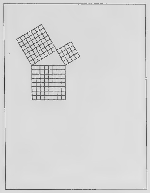Transparency 9-5-2: Converse of the Pythagorean Theorem

halves of the hexagon.

Next, move the two quadrilateral pieces to the side of the figure and call attention to the hexagon that contains the square c² and the two triangles above and below it. What kind of symmetry does it seem to have? (Rotation.) Draw a line through the vertices of its two right angles and place the two plastic pieces to fit the two quadrilateral halves of this hexagon.

It is possible to prove what the two arrangements of the plastic pieces suggest—that the two hexagons have equal areas. Remove the plastic pieces and call attention again to the regions contained in each hexagon. How does it follow from the fact that the hexagons havae equal areas that a² + b² = c2? (The extra triangles are copies of the original triangle, and so they have equal areas. Letting the area of one of the triangles be x, we have

a² + b²+2x =c*+2x and so

a² +b² =c²,)

To introduce the converse of the Pythagorean Theorem, show Transparency 9-5-2 and explain that this figure is a triangle in which squares have been drawn on the three sides. Then ask if it is a right triangle. If c² a² + b², does it follow that a triangle is not a right triangle? (Yes. Suppose that the triangle is a right triangle. Then c² = a² + b², which contradicts the hypothesis. So it is not a right triangle.) Now suppose that for the triangle on Transparency 9-5-2 we have found that c² = a² + b². Could we conclude from the Pythagorean Theorem that the triangle is a right triangle? (No. We would be

making the converse error.) This raises the question of whether the converse of the Pythagorean Theorem is true. Remark that it is and that the proof is left as one of the exercises.

I recommend giving two assignments on this lesson, limiting the first assignment to some or all of the exercises of Set I.

Second day

Introduction

Every year the Nile River in Egypt overflows its banks in late summer and floods the surrounding land. Herodotus, a Greek historian of the fifth century B.C., wrote: When the Nile inundates the land all of Egypt becomes a sea, and only the towns remain above water, looking rather like the islands of the Aegean. At such times shipping no longer follows the stream, but goes straight across the country.

Because the flooding wiped out many boundary lines, the ancient Egyptians developed some of the basic principles of surveying to reestablish them. The picture on Transparency 9-5-3 is part of a mural more than 3,000 years old. It shows surveyors holding a rope with knots equally spaced along it. By stretching the rope out to form a triangle, the surveyors made use of something we considered in yesterday’s lesson.

The following makes a nice demonstration. Take a rope about 25 feet long and put 13 knots in it at 2-foot intervals. Give a knot at one end to a student to hold and form, in the middle of your class, a 3-4-5 triangle by having other students hold the ap-

Transparency 9-R-1

Transparency 9-R-2: Map: Manhattan

Transparency 9-R-3: The area of a human being

Transparency 9-R-2: Map: Manhattan

propriate knots. Do not tell the class what lengths the sides of the triangle are, but let the students observe them for themselves. The sides should be stretched out tight and the students outside the triangle should stand up and look at the result. Let a student explain what he or she observes. Note that we know that a 3-4-5 triangle is a right triangle not because of the Pythagorean Theorem but because of its converse. A nice transparency could be made from the photograph of an Egyptian field divided into squares from Ancient Egypt by Lionel Casson, in the Great Ages of Man series (Time-Life Books, 1965), pages 48-49. The caption to this photograph is especially appropriate:

A panorama of applied geometry, this Egyptian

field is a patchwork of small squares criss-

crossed with irrigation canals and ditches. To

sustain agriculture in an arid land, the people had to become engineers and learn how to construct complex irrigation works. To cope with the confusion caused by the annual flood of the Nile, Egyptians worked out the rudiments of geometry. “Rope-stretchers,” or surveyors, applied the methods of geometry to redraw the property lines obscured during the flood. Thus the needs of agriculture led the ancient Egyptians to become more than good farmers: mastering both the desert and the river, they not only achieved new skills but expanded their intellectual horizons in the process.*

“Ancient Egypt by Lionel Casson (Time-Life Books, 1965), pages 48-49.

Review of Chapter 9

First day

Transparencies

• 9-R-1 _ The Flatiron building
• 9-R-2 Map: Manhattan
• 9-R-3 The area of a human being
• 9-R-2 Table: A person’s area

Introduction

Most of the streets of Manhattan intersect each other at right angles, as they do in most cities. One street that does not, however, is Broadway. The photograph on Transparency 9-R-1 was taken in 1903 at the spot where Broadway (on the left) intersects Fifth Avenue. As the picture shows, the two streets meet at a rather sharp angle and, on the property at the corner, one of the city’s first skyscrapers was built. The building, popularly known as the Flatiron Building, still stands at this intersection.

The map on Transparency 9-R-2 shows the plot of land on which the Flatiron Building was constructed. It is in the shape of a triangle whose sides have lengths 80 feet, 150 feet, and 170 feet. What is the area of the land on which the Flatiron Building stands? (80? + 150? = 1702, so the triangle is a right

1 triangle. Its area is 3 (80)(150) = 6,000 square feet.)

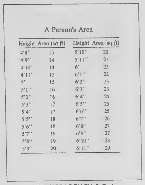Transparency 9-R-4: A Person’s Area

Second day

Introduction

Almost everyone knows their height and weight quite accurately. Do you know, on the other hand, what your area is? (Show Transparency 9-R-3.) By this, I mean the total surface area of your skin. The lower figure represents the skin of the person in the upper figure stretched out flat like a pelt.

We have developed formulas for finding the areas of a variety of geometric figures, but they are of no use in finding the area of a figure as complex as this. The area of a person of average weight and body build depends on his or her height. Make an estimate of your own area and then I will give you a formula by means of which you can determine it more accurately. (It might be fun to have your students write their estimates on scraps of paper, and then collect the estimates and read some of the more extreme ones to the class before going any further.)

You can find your approximate area by means of the following formula:

3

aod

é )

in which h is your height in feet. After your students have had time to compute their areas by this formula, show Transparency 9-R-4 so that they can check their answers. Each area is rounded to the nearest square foot.

Transparency 10-1-1: Photographs of Winnie Mae and models

Transparency 10-1-2: Diagrams of Winnie Mae

Transparency 10-2-1: Betty Grable

Chapter 10: Similarity

Lesson 1: Ratio and Proportion

Lesson Outline

Terms: Ratio, proportion, terms, means, extremes, geometric mean.

Transparencies

• 10-1-1 Photographs of Winnie Mae and models
• 10-1-2 Diagrams of Winnie Mae

Introduction

One of the airplanes in the pictures on Transparency 10-1-1 is an exact replica of the first plane to be flown on a solo flight around the world. Its pilot was Wiley Post and the year was 1933. Although the other plane looks exactly like Post’s plane, it could never be flown around the world because it is too small: it is a scale model of the real plane and weighs only 15 pounds. Can you guess which plane is which? (The one pictured at the top is the model.)

To be convincing, the model must have the same shape as the actual plane. Hand out duplicated copies of Transparency 10-1-2 and explain that the figures could represent views of either the plane or the model. Have your students write the letters w and I on the figures to represent wingspan and length. The plane is 27 ft long and has a wingspan of 42 ft. The model is 4.5 ft long. Can you find out what its wingspan is? (Give your students time to think about this and then let some of those who have the correct answer−7 ft—explain their methods.)

Use the proportion

ON ee

BSS 27, to review the meanings of “ratio” and “proportion,” and present the rest of the lesson as in the text.

Lesson 2: Similar Figures

Lesson Outline

Terms: Similar triangles, similarity correspondence, center and magnitude of a dilation.

Transparencies

• 10-2-1 Betty Grable
• 10-2-2 Why slide enlargements have wrong

proportions 10-2-3 Slide frame and an 8 x 10 photograph

Introduction

Show Transparency 10-2-1. (If your school has a photography class, you might ask a student to take a photograph of one of your school’s well-known athletes—for example, a member of the basketball, baseball, football, gymnastic, soccer, or wrestling teams. Be sure that the photograph is clear enough so that your class can make the required measurements with accuracy.) The Renaissance artist Albrecht Diirer wrote several books on human proportions. Add the overlay. (Make a new overlay if you use a photograph of a student in your school.

Transparency 10-2-3: Slide frame and an 8 x 10 photograph

Transparency 10-2-2: Why slide enlargements have wrong proportions

The overlay should mark the positions of the neck, hip, knee, and ankle.) In one of his books, Durer claimed that for most people, the distance from hip to knee is the geometric mean between the distance from neck to hip and the distance from knee to ankle.*

The lines on this photograph of the actress Betty Grable (the “pin-up” girl of World War II), mark the positions of these four points: neck, hip, knee, and ankle. Place an ordinary centimeter ruler on the picture and measure the distance between hip and knee and the distance between knee and ankle, each to the nearest tenth of a centimeter. (They are 5.6 cm and 4.7 cm, respectively.) Mark the distances on the picture and ask your students to use their calculators to figure out what the distance from knee to

hip should be if Dürer’s claim is correct. (x/5.6 = 5.6/4.7; x = 6.7.) Measuring this distance on the picture will reveal that Dürer’s statement seems to be true.

Alternative Introduction Show Transparency 10-2-2, keeping the answer to the question covered. This question once appeared in a photography column in the Los Angeles Times. Read it to your class and, still keeping the answer covered, remark that the answer to the question is the subject of the new lesson.

Hand out duplicated copies of Transparency 10-2-3, on which a 35-mm slide in a frame and an

8 x 10 print are represented. The print is drawn in centimeters rather than inches so that it will fit on the transparency. When a picture is enlarged, it and its enlargement have the same shape. Figures that have the same shape are similar. Define similar triangles and then explain that the definition can be extended to rectangles. Point out that the problem with the slide enlargement is obviously not with the angles. Have your students measure the inner dimensions of the frame in millimeters. (They are about 23 mm and 33 mm, the frame being slightly smaller than the picture on the 35-mm film.)

If the slide is enlarged to a width of 80 mm (8 cm), what will its length be? (23/80 = 33/x; x = 115.) The picture will be approximately 11.5 cm long and this is the cause of the problem. Have your students extend the rectangle representing the print downward another 1.5 cm to show the part of the picture that got eliminated.

To avoid losing part of the picture, the slide could be enlarged to a length of 100 mm instead. In

this case, what would its width be? (x/100 = 23/33; x ≈ 70.) The picture would be approximately 7 cm wide.

Put Transparency 10-2-2 back on the screen and read the first paragraph of the answer, whose meaning will now be very clear.

*Dan Pedoe devotes an entire chapter of his book Geometr y and the Liberal Arts (St. Martin’s Press, 1976) to the geometry of Dürer.

Transparency 10-3-1: Side view of the Grande Dixence dam

Transparency 10-3-2: Side-splitter theorem figures

Transparency 10-4-1: “How to build a house quickly”

Lesson 3: The Side-Splitter Theorem

Lesson Outline

Theorem 44. The Side-Splitter Theorem. If a line parallel to one side of a triangle intersects the other two sides in different points, it divides the sides in the same ratio. Corollary. If a line parallel to one side of a triangle intersects the other two sides in different points, it cuts off segments proportional to the sides.

Transparencies

• 10-3-1 Side view of the Grande Dixence dam
• 10-3-2 Side-splitter theorem figures

Introduction

Show Transparency 10-3-1. The photograph shows the Grande Dixence dam in the Swiss Alps, one of the highest dams in the world. The dam was completed in 1961 at a cost of 372 million dollars and holds back more than ten million tons of water.

Explain the meaning of the figure below the photograph (see page 392 of the text). Then present the problem of finding the length of EC indirectly from the lengths of AD, DB, and AE as is done in the text. The figure on the transparency is drawn on a somewhat different scale from that of the one shown in the text. Tell your students that 1 cm on the figure represents a distance of 70 m and measure AD, DB, and AE, expressing each length in meters. (They are 70 m, 280 m, and 105 m, respectively.) Ask your students if they can figure out the length of EC before you measure it and have someone who finds the length explain how he or she did it.

Hand out duplicated copies of Transparency 10-3-2 for your students to use in developing the proof of the Side-Splitter Theorem.

Lesson 4: The AA Similarity Theorem

Lesson Outline

Theorem 45. The AA Theorem. If two angles of one triangle are equal to two angles of another triangle, the triangles are similar. Corollary. Two triangles similar to a third triangle are similar to each other.

Transparencies

• 10-4-1 “How to build a house quickly”
• 10-4-2 Walking in the house
• 10-4-3 AA Similarity Theorem figures
• 10-4-4 How to measure up by looking down

First day

Introduction

The following exercise is based on a problem in a fascinating book titled Children Solve Problems by Edward de Bono (Harper and Row, 1974). Children of various ages were asked to solve problems such as how to stop a cat and dog from fighting, how to weigh an elephant, and how to build a house quickly.

One boy, when given the problem of how to build a house quickly, drew the diagram on Transparency 10-4-1. He figured that, because toy houses are sometimes made by cutting and folding cardboard, the same method might be applied to constructing a house from sheet metal. One problem with his solution is the design that he proposes.

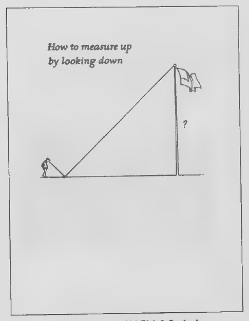Transparency 10-4-4: How to measure up by looking down

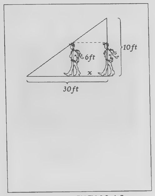Transparency 10-4-2: Walking in the house

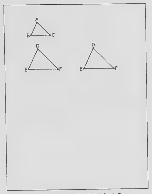Transparency 10-4-3: AA Similarity Theorem figures

Show Transparency 10-4-2. The roof of the house slants down to one side so that someone walking in the front door would soon bump his head on the ceiling.

Suppose that the right-hand wall of the house as shown here is 10 feet high and that the house is 30 feet wide. (The figure is not drawn to scale.) How far do you think a person 6-feet tall could walk before his head would touch the ceiling?

There are three triangles in the figure, all of which look as if they might be similar. If they are, we can write a proportion between their sides, such as

slice Ehed

10 30 10 30

to find that the person could walk 12 feet.

This raises the question of whether the triangles in the figure are really similar. Remind your students that we never bother to show that all six pairs of parts of two triangles are equal to prove that they are congruent. Certain sets of three pairs of parts are sufficient. (Ask someone to name them.) Then tell your students that it is even easier to prove that two triangles are similar. All we have to show is that two pairs of angles are equal.

Hand out duplicated copies of Transparency 10-4-3 for use in proving the AA Similarity Theorem as in the text. The corollary to this theorem should also be considered before returning to the figure on Transparency 10-4-2 to see why the three triangles are similar. The two smaller triangles are similar to the large one because of the AA Similarity Theorem (the triangles have equal right angles

and common angles); they are similar to each other because of the corollary to the AA Theorem.

If you plan to do the height-measuring experiment on the next day, you might limit the assignment to selected exercises from Set I of Lesson 4.

Second day

Introduction

If possible, take your class outside and let your students try to measure the height of your school flagpole or a tree by means of the mirror method illustrated on Transparency 10-4-4. You need some small mirrors (one for every three students), at least one 50-ft tape measure, and some shorter tape measures. I assign my students to groups of three each: one student in each group acts as the observer, one as the measurer, and one as the recorder. Note that the method assumes that the feet of the observer, the mirror, and the base of the pole or tree are in a hortzontal plane and also that the mirror is level. You might ask your students why these things are important. (They are necessary if the angles in the two triangles are to be equal; this, of course, is the basis for our treatment of them as similar when we write a proportion between their pairs of corresponding sides.)

Although the students work in small groups, I hold each student responsible for making and turning in his or her own calculations.

Some more exercises from Lesson 4 might be assigned for homework.

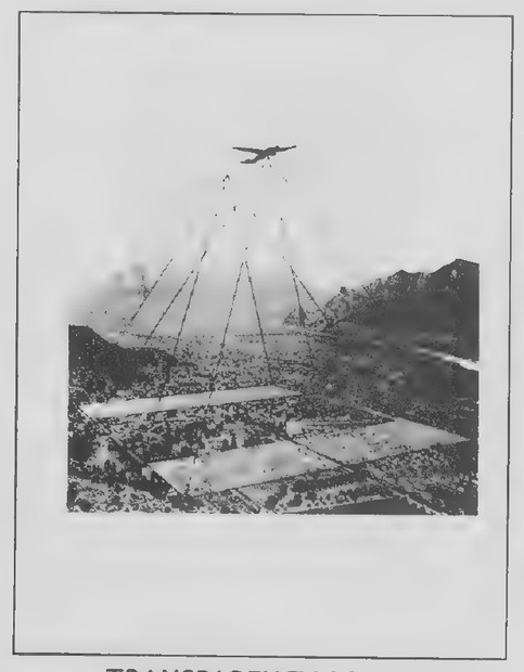Transparency 10-5-1: Aerial photography

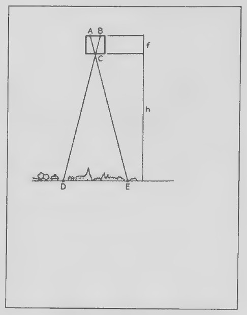Transparency 10-5-2: Aerial-photography scale diagram

Transparency 10-6-1: An early medical x-ray

Lesson 5: Proportions and Dilations

Lesson Outline

Terms: Corresponding altitudes. Theorem 46. Corresponding altitudes of similar triangles have the same ratio as that of the corresponding sides.

Transparencies

• 10-5-1 Aerial photography
• 10-5-2 Aerial-photography scale diagram

Introduction

Show Transparency 10-5-1. Aerial photography plays an important part in modern map-making. The plane carrying the camera flies on a straight course parallel to the ground and the camera takes a continuous series of overlapping pictures. The figure on the transparency shows the overlap of two successive photographs taken in flight.

It is important to know what the scale of the pictures produced is—that is, how the dimensions of the photograph compare with the dimensions of the region being photographed. The diagram on Transparency 10-5-2 shows how this scale is determined. The figure at the top represents the camera: C is the lens, AB is the film, and fis the focal length of the lens. The altitude of the camera is h and the part of the ground picked up on the film is DE.

Given that AB ∥ DE, why does it follow that △ABC ∼ △EDC? Although f and h are not lengths of sides of these triangles, they are lengths of corresponding altitudes. We can prove that corresponding altitudes of similar triangles have the same ratio as that of the corresponding sides.

After developing this proof, go back to Transparency 10-5-2. The scale of the photograph illus-

trated in this diagram is ≅ Because we have

proved that corresponding altitudes of similar triangles have the same ratio as that of the corresponding sides, we can conclude that

This provides the way by which the scale of aerial photographs is determined: it is found by dividing the focal length of the lens by the altitude of the camera. For example, a camera with a focal length of 6 inches and an altitude of 2 miles produces photographs with a scale of

6 in 0.5 ft 1 1

2mi 2(5,280) ft -4(5,280) 21,120°

Lesson 6: Perimeters and Areas of Similar Figures

Lesson Outline

Theorem 47. The ratio of the perimeters of two similar polygons is equal to the ratio of the corresponding sides.

Theorem 48. The ratio of the areas of two similar polygons is equal to the square of the ratio of the corresponding sides.

Transparencies

• 10-6-1 An early medical x-ray
• 10-6-2 X-ray of bird shot in hand
• 10-6-3 X-ray diagram

Transparency 10-6-2: X-ray of bird shot in hand

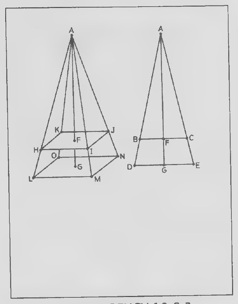Transparency 10-6-3: X-ray diagram

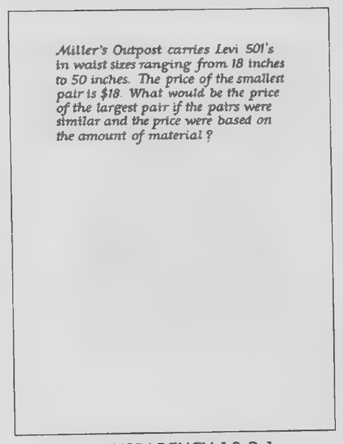Transparency 10-R-1: Levi 501’s

Introduction

The photograph on Transparency 10-6-1 was taken at Dartmouth College in 1896 and shows one of the medical uses of x-rays. The patient, sitting with his back toward the camera, is having his broken arm x-rayed. The doctors taking the x-ray were not yet aware of the dangers of prolonged radiation.

The x-ray photograph on Transparency 10-6-2 was taken in the same year and shows bird shot that became embedded in the patient’s hand in a hunting accident.

When an x-ray photographis taken, itis always larger than the object it pictures. The reason for this can be seen from the figures on Transparency 10-6-3. In the first figure, a three-dimensional view, the source of the x-rays is at A, the object being photographed is shown as the upper rectangle, and its image on the photographic plate is shown as the lower rectangle. The second figure is a two-dimensional view.

To emphasize the connection between the two figures, have your students add segments BC and DE to the first figure. How does it follow from the fact that BC ∥ DE that △ABC ∼ △ADE in the second figure? Given that AF ⊥ BC, AG ⊥ DE, AF = 16 cm, and FG = 4 cm, find BC/DE. (Because corresponding altitudes of similar triangles have the same ratio as the corresponding sides, BC/DE = AF/AG = 16/20 = 4/5.) This means that the dimensions of the object being x-rayed are four-fifths the corresponding dimensions of the image in the photograph.

If the area of the image in the photograph is 50 cm², what is the area of the object x-rayed? To answer this question, we have to know something about the areas of similar polygons.

Use triangles as on pages 415-416 of the text to prove the perimeter and area relations for similar polygons and then repeat the question about the area of the x-ray. It can be proved that HIJK ∼ LMNO. Therefore, αHIJK/αLMNO = (HI/LM)². Because BC = HI and DE = LM, we can conclude that αHIJK/αLMNO = (BC/DE)². If αLMNO = 50 cm², find αHIJK. [Letting αHIJK = x, we have x/50 = (4/5)² = 16/25, from which it follows that x = 32.] The area of the object x-rayed is 32 cm².

Review of Chapter 10

Transparencies

• 10-R-1 Levi 501’s
• 10-R-2 Eclipsing the moon with a dime

First day

Introduction

The problem on Transparency 10-R-1 provides a review of the theorem about the areas of similar polygons. Because some students are likely to immediately conclude that the answer is $50, you may want to warn them that this is wrong. Let a student who finds the correct answer explain his or her method. (If the price is based on the amount of ma-

Transparency 10-R-2: Eclipsing the moon with a dime

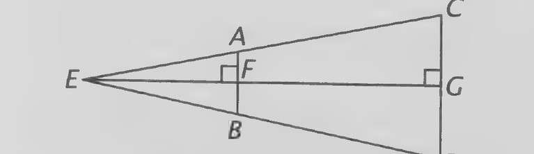Figure on page 366 — Similar right triangles used to measure an inaccessible distance (points A, B, E, F marked)

terial, we need to compare the areas of the cloth used in making each pair of pants. If they are similar and x represents the price of the largest pair, 18/x = (18/50)²; x = 138.89.) The largest pair would cost about $139. After finishing the problem, you might point out that, although it seems reasonable to assume that clothing patterns over a small range of sizes are similar to each other, the assumption in the problem that the smallest and largest pairs of Levi’s are similar is not very plausible.

Second day

Introduction

Show Transparency 10-R-2. Imagine that you are standing outside on a night in which there is a full moon. If you closed one eye and held a dime directly in front of your other eye, you could easily “cover” the moon with it. In other words, held close to your eye, the dime would appear larger than the moon. Now suppose that you move the dime away from your eye and toward the moon. How far away do you think you would have to hold the dime in order for it to appear to be the same size as the moon? Six inches? A foot? Students who have dimes with them might hold the coins at various distances from their eyes before guessing the answer to this problem.

Have your students draw the figure shown at the right and explain that point E represents your eye; AB, the edge of the dime; and CD, the edge of the “disk of the moon.” If the dime is held so that AB ∥ CD, then △EAB ≅ △ECD. Because the distances

from your eye to the dime and moon are the lengths of the corresponding altitudes (EF and EG) of these triangles, we know that EF/EG = AB/CD. Which of the four lengths in this proportion is the answer to the question? What do the other lengths represent? EG, the distance to the moon, is about 385,000 km and CD, the diameter of the moon, is about 3,480 km. Students with dimes can measure AB, which is about 1.8 cm. By substituting, we get

EF/385,000,000 m = 0.018 m/3,480,000 m, and so EF ≈ 2 m.

The distance from your eye that you would have to hold the dime in order that it would look equal in size to the moon is about two meters—much farther than anyone would be capable of actually holding it!

Transparency 11-1-1: Photograph of chambered nautilus

Transparency 11-2-1: The Pythagorean Proposition

Transparency 11-2-2: Photograph of Elisha S. Loomis

Chapter 11: The Right Triangle

Lesson 1: Proportions in a Right Triangle

Lesson Outline

Terms: Projection.

Theorem 49. The altitude to the hypotenuse of a right triangle forms two triangles similar to it and to each other.

Corollary 1. The altitude to the hypotenuse ofa right triangle is the geometric mean between the segments into which it divides the hypotenuse. Corollary 2. Each leg of a right triangle is the geometric mean between the hypotenuse and its projection on the hypotenuse.

Transparencies

• 11-1-1 Photograph of chambered nautilus

Introduction

A chambered nautilus shell cut in half so that the compartments can be seenis an attractive visual aid to have for the mathematics classroom and is worth looking for. The photograph on page 428 of the text is of a shell that can be bought for just a few dollars at an oceanside store.

The chambered nautilus is most abundant in the southwest Pacific where it swims on the ocean floor in search of food. The nautilus lives in the outermost chamber of its shell and can let air into or out of the other chambers to help in moving upward or downward through the water.

Show Transparency 11-1-1 and mark and label the center point of the shell point P. Have a student draw a line through point P in any direction and a second line through P that is perpendicular to the first. Then, label some of the consecutive points in which the curve of the shell intersects these lines and develop the rest of the lesson as presented on pages 428-429 of the text.

Lesson 2: The Pythagorean Theorem Revisited

Lesson Outline

Theorem. The Pythagorean Theorem. Ina right triangle, the square of the hypotenuse is equal to the sum of the squares of the legs.

Transparencies

• 11-2-1 The Pythagorean Proposition
• 11-2-2 Photograph of Elisha S. Loomis
• 11-2-3 Page from The Pythagorean Proposition

Introduction

Dr. Elisha Loomis taught mathematics at West High School in Cleveland, Ohio, from 1895 to 1923. As one of his hobbies, he collected proofs of the Pythagorean Theorem. Three hundred and seventy of these proofs were published in a book whose title page is shown on Transparency 11-2-1.* A picture

*The Pythagorean Proposition by Elisha Scott Loomis (privately printed in 1927 and 1940; reprinted in 1968 as volume 1 of N.C.T.M’s Classics in Mathematics Education series).

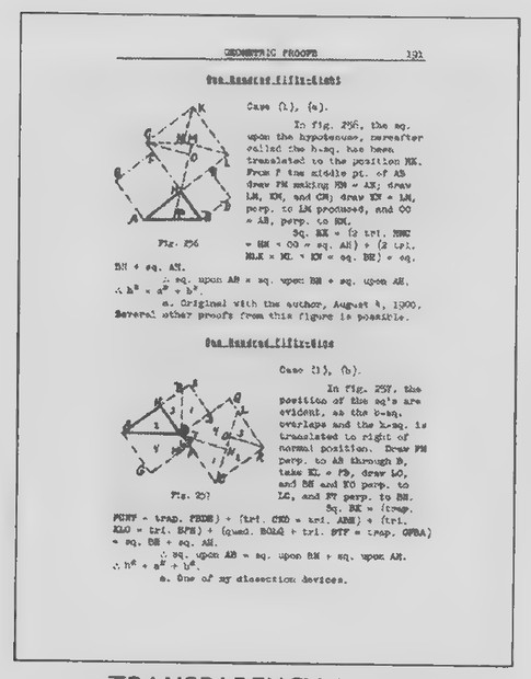Transparency 11-2-3: Page from The Pythagorean Proposition

Transparency 11-3-1: A Pythagorean guitar

Transparency 11-3-2: Cover of The Square of the Hypotenuse

of Dr. Loomis is on Transparency 11-2-2 and a typical page from the book is shown on Transparency 11-2-3.

In our previous encounter with the Pythagorean Theorem, we considered several proofs based on area. The exercises also emphasized the area aspect of the theorem. In this lesson, we concentrate more on how the Pythagorean Theorem is used to find lengths. We begin with an unusually simple proof of it based on a theorem of yesterday’s lesson. Guide your students in writing the proof presented on page 435 of the text.

Lesson 3: Isosceles and 30°-60° Right Triangles

Lesson Outline

Theorem 50. The Isosceles Right Triangle Theorem. In an isosceles right triangle, the hypotenuse is ¥2 times the length of a leg.

Corollary. Each diagonal of a square is -/2 times the length of one side.

Theorem 51. The 30°-60° Right Triangle Theorem. In a 30°-60° right triangle, the hypotenuse is twice the shorter leg and the longer leg is V3 times the shorter leg.

Corollary. An altitude of an equilateral triangle 13 having side s is * and its area is aie

Transparencies

11-3-1_ A Pythagorean guitar 11-3-2 Cover of The Square of the Hypotenuse 11-3-3 First page from The Square of the Hypotenuse

Introduction

In his book, The Number of Things: Pythagoras, Geometry and Humming Strings (Dutton, 1964), Evans G. Valens describes a “Pythagorean guitar” that your students will find especially interesting. The guitar, pictured on Transparency 11-3-1, is easy to build. All you need is a guitar string, a piece of wood, two nails, two small pulleys (to equalize the tension), and a set-screw.

If a guitar string is stretched around three nails at the vertices of a 3-4-5 right triangle, the three sides of the string triangle, when plucked, will sound a musical chord. If the hypotenuse is tuned to G, the longer and shorter legs will sound B and E, respectively. Valens notes that these are the top three strings of a guitar and that the chord sounded is a minor triad. If arandomly shaped “triangle guitar” is played, it will not ordinarily produce a musical chord. Why does the 3-4-5 right triangle do so? Because Pythagoras, as well as being a great mathematician, was also the founder of the science of music. His belief in the importance of whole numbers led him to define the intervals in the musical scale in terms of them. The scales of Pythagoras are discussed in great detail in chapters 14 through 16 of Valens’s book.

A song that would be especially appropriate to play on a Pythagorean guitar was once featured in a Hollywood movie (Merry Andrew, M-G-M Pictures, 1958). Its title is “The Square of the Hypotenuse” and the cover and first page of the sheet music are pictured on Transparencies 11-3-2 and 11-3-3.

In presenting the new lesson on the relations of

Transparency 11-3-3: First page from The Square of the Hypotenuse

Transparency 11-4-1: Crazy inventions

Transparency 11-4-2: A device for preventing train collisions

the lengths of the sides of isosceles and 30°-60° right triangles, you should mention that these theorems are very important in trigonometry as well as geometry.

Lesson 4: The Tangent Ratio

Lesson Outline

Terms: Tangent ratio

Transparencies

• 11-4-1 Crazy inventions
• 11-4-2 A device for preventing train collisions

Introduction

Some extraordinary inventions have been patented in the U.S. Patent Office. A book titled Absolutely Mad Inventions by A. E. Brown and H. A. Jeffcott, Jr. (Dover, 1970) contains reproductions of the original drawings and descriptions filed for some of these patents.

Two of them are shown on Transparency 11-4-1. The first is a pair of goggles for a chicken, to protect its eyes in case other chickens peck it in the head. The second, a device for catching fish, is rather quaintly described by its inventor in these words:

The fish B, when approaching the bait s, will see

the reflection B’, of himself in the mirror, also

coming for the reflection of the bait s’, and will

be made bolder by the supposed companionship,

and more eager to take the bait before his com-

petitor seizes it. He will lose his caution, and take

the bait with a recklessness that greatly increases

the chances of his being caught on the hook.

Another remarkable invention is one for preventing train collisions. It was registered in 1895 and is pictured on Transparency 11-4-2. If a train meets another one approaching on the same track, it can run up the slanted rails of a special car, along rails on top of the rest of the cars, and down the other end car. Instead of colliding, one train merely passes over the other! If two trains are traveling in the same direction, one can overtake and pass the other by the same procedure.

The figures reveal that the end cars are approximately right triangular in shape. If the box cars on the train are 14 ft high and the track on one of these end cars rises at a 15° angle with the horizontal, how long must the car be?

If the angle were 30° or 45°, we could use one of the theorems of the last lesson to find the answer. Because it is not, we need to use some other method. (Following this introduction, you can introduce the tangent ratio and show how it can be used to find the length of one of these end cars. Your students will need some guidance, of course, in learning how to find tangents and inverse tangents on their calculators. Letting x = the length, we have tan 15° = 14/x, from which it follows that x ≈ 52.2 ft. For a rise of 15°, the end car would be about 52 feet long.)

Transparency 11-5-1: Overhanging-rock photograph

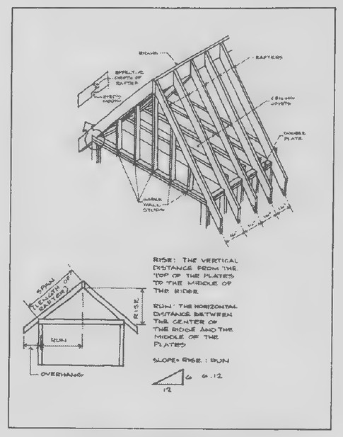Transparency 11-6-1: Rafters and slope

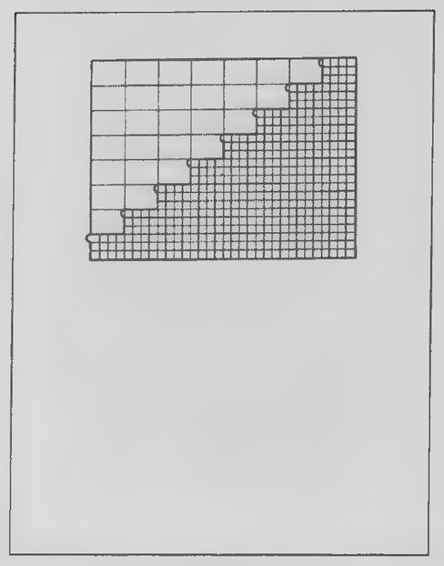Transparency 11-6-2: Staircase

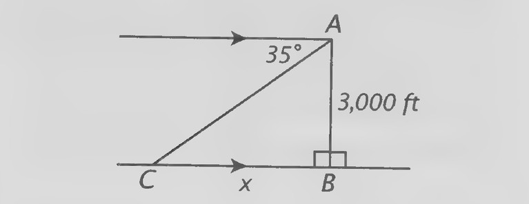Figure on page 370 — Measuring a height from a distance: an angle of elevation of 35° and a horizontal distance of 3,000 ft

Lesson 5: The Sine and Cosine Ratios

Lesson Outline

Terms: Sine ratio, cosine ratio

Transparencies

• 11-5-1 _ Overhanging-rock photograph

Introduction

The two women in the photograph on Transparency 11-5-1 are dancing on Overhanging Rock at Glacier Point in Yosemite. The picture was taken in 1900, many years before the National Park Service decided that such stunts were too dangerous and barred access to the rock.

Overhanging Rock is 3,000 feet above the valley floor. Suppose that you are standing on the rock and looking down at a point in the valley such that the angle of depression of that point from your position is 35°. (Have your students draw a figure like the one shown here to illustrate this.) How far is

the point of the rock? After your students have had some time to work on this, have someone explain his or her solution. Note that the problem can be solved by either

of the following equations:

= x 6 ℓ03,000

tan 55 = 3,000 or tan35 His

The answer is approximately 4,300 feet.

To introduce the new lesson, ask how far the point you are looking at is from you (label this distance y in the diagram). To find the answer, we can use either the Pythagorean Theorem or another trigonometric ratio. Define the sine and cosine ratios and show how the problem can be solved by using either ratio. The answer is approximately 5,200 feet.

Lesson 6: Slope

Lesson Outline

Terms: Run, rise, slope, angle of inclination, slope.

Theorem 52. Two nonvertical lines are parallel iff their slopes are equal.

Theorem 53. Two nonvertical lines are perpendicular iff the product of their slopes is -1.

Transparencies

• 11-6-1 Rafters and slope
• 11-6-2 Staircase

Introduction

In designing the roof of a building, the architect has to take into account the forces of wind, rain, and snow. If the roof is very steep, for example, snow will tend to slide off it. If the slope is more gentle, snow will remain where it is, so that the roof must be able to support the resulting weight. The figures on Transparency 11-6-1 are from the chapter on roof

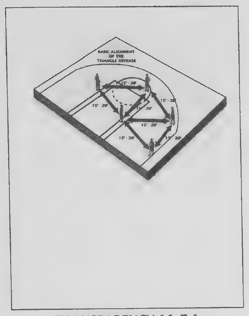Transparency 11-7-1: The triangle offense

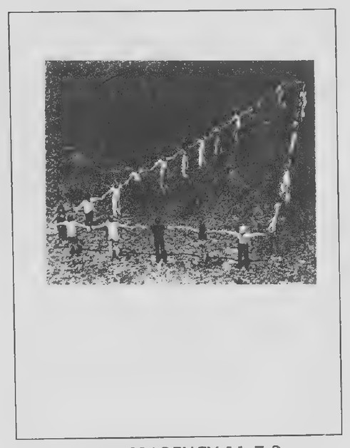Transparency 11-7-2: Human triangle in Japan

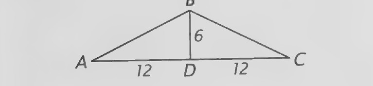Figure on page 371 — A triangle with its altitude drawn, the height marked 6 and the base divided into segments 12 and 12

design in the book How to Design and Build Your Own House by Lupe DiDonno and Phyllis Sperling (Knopf, 1981). It is interesting to note that the architect and the mathematician use the same terms in discussing slope. With this introduction, you might have your students make a scale drawing on graph paper to represent a roof whose rafters match the 6:12 diagram at the bottom of the transparency. This figure can be used as a basis for developing the rest of the lesson.

B

slope in architecture is in the design of stairways. The figure on Transparency 11-6-2 shows the steepest stairway allowed by most building codes in the United States. What is its slope? It is interesting to note that itis based on the 3-4-5 right triangle, so that its slope

1S 4

Lesson 7: The Laws of Sines and Cosines

Lesson Outline

Theorem 54. The Law of Sines. If the sides opposite ∠A, ∠B and ∠C of △ABC have lengths a, b, sin A sinB _ sin C and c, then b Cc

Theorem 55. The Law of Cosines. If the sides

opposite ∠A, ∠B and ∠C of △ABC have

lengths a, b, and c, then c² = a² + b² — 2ab cos C.

Transparencies

• 11-7-1 The triangle offense
• 11-7-2 Human triangle in Japan

First day

Introduction

Because there is a lot to cover in this lesson, I recommend that you begin class by using Transparency 11-7-1 to introduce and present the lesson as in the text.

Second day

Introduction

The photograph on Transparency 11-7-2 was taken by Ronald L. Dirkse of the American School in Tokyo, Japan. It shows a group of students standing on the football field with their arms outstretched to form the sides of a large triangle. The side of the triangle closest to the camera is formed by five students; 12 students and 13 students stand along the other two sides. If all of the students are the same size, what kind of triangle do you suppose is formed? (Students who recognize that “5-12-13” is a Pythagorean triple will immediately recognize that the triangle is a right triangle. Those who do not can verify that 5¢ + 122 = 132, from which we can draw the same conclusion from the converse of the Pythagorean Theorem.)

Now suppose that one more student joins the group, so that the shortest side of the triangle increases from 5 to 6. What kind of triangle would

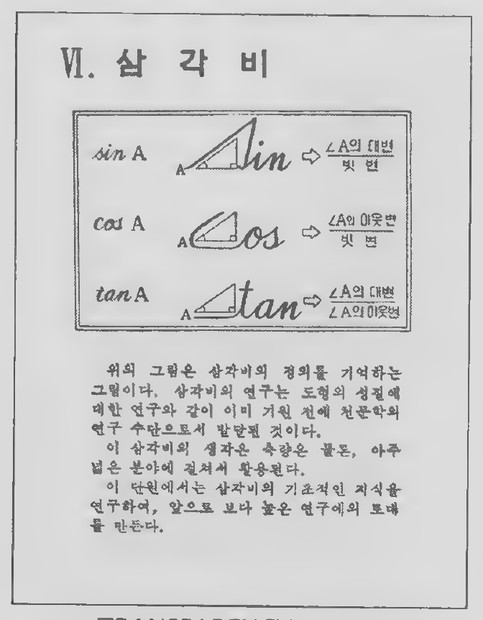Transparency 11-R-1: Trigonometric ratios from a Korean geometry book

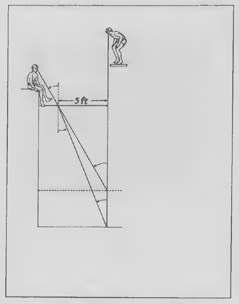Transparency 11-R-2: Swimming-pool refraction problem

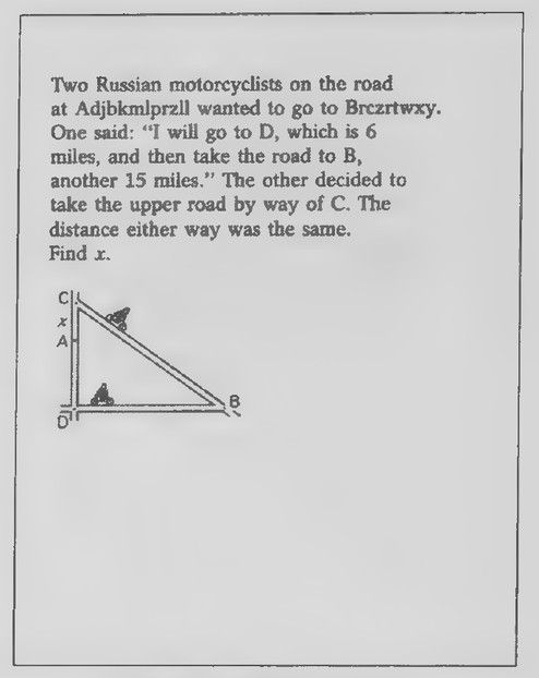Transparency 11-R-3: Russian motorcyclists problem

result? (You might take a poll of your students to find how many think that the triangle would become acute and how many think it would become obtuse.) Which would you use, the Law of Sines or the Law of Cosines, to find the measures of the angles of a triangle, given its sides? (The Law of Cosines.) Why? (To write a proportion from the Law of Sines requires that we know at least one angle of the triangle, but we do not.) Which angle of the triangle do we need to determine to be able to tell whether the triangle is acute or obtuse? (The largest angle.) Letting C be the vertex of the largest angle, write an equation for the triangle based on the Law of Cosines. [13? = 6? + 122 — 2(6)(12)cos C.] Solve the equation to find out if you guessed correctly as to what type a 6-12-13 triangle is. (Solving

the equation for cos C, we get cos C = = from

which ∠C = 85.6°. The triangle is acute.)

Having done this, you might have your students construct a triangle with sides of 6 cm, 12 cm, and 13 cm, so that they can measure its largest angle with their protractor to confirm that their calculations are reasonable.

Review of Chapter 11

First day

Transparencies

• 11-R-1 Trigonometric ratios from a Korean

geometry book 11-R-2 Swimming-pool refraction problem 11-R-3 Russian motorcyclists problem 11-R-4 Gurus problem

Introduction

Transparency 11-R-1 shows a page from a Korean mathematics book. Your students will be interested in seeing the device used to help in remembering the definitions of the trigonometric ratios. It is clever, but surprising, because it is based on the script forms of letters of the Latin alphabet! Note that our knowledge of the definitions makes it possible to translate the Korean symbols inside the large box.

The figure on Transparency 11-R-2 illustrates refraction of light in a swimming pool.* The two observers are looking at a stone at the bottom of the pool. The observer on the diving board is looking directly down at the stone. The observer at the left sees the stone from the side. Light from the stone is bent at the surface of the water, producing the illusion that the bottom of the pool is higher than it actually is.

Hand out duplicated copies of the transparency and have your students label the angle above the surface of the water 30° and the angle just below the surface 22°. The problem is to use this information to find the actual depth of the water in the swimming pool (label this x on the figure) and the apparent depth of the water as seen by the observer sitting on the side of the pool (label this y).

Applying the tangent ratio to the right triangles

in the figure, we get tan’22° = Es ta=sL2.4 and

x

“The figure and the description given in this lesson are taken from Introductory Physics by Mashuri L. Warren (W. H. Freeman and Company, 1979).

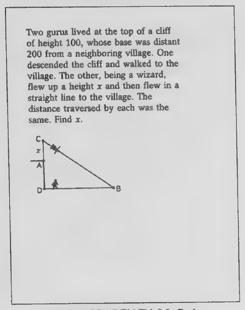Transparency 11-R-4: Gurus problem

5 tan 30° = —, y= 8.7. The water is actually 12.4 feet deep, whereas to the observer on the left, it appears to be 8.7 feet deep.

Second day

Introduction

The puzzle of the Russian motorcyclists on Transparency 11-R-3 appeared in a book published in England in 1926 (Modern Puzzles by Henry Ernest Dudeney). Your students may need some help in writing and solving the equation on which the solution is based.

After discussing the solution, show Transparency 11-R-4. The puzzle of the motorcyclists bears an interesting resemblance to this puzzle, which was invented by the Hindu mathematician Brahmagupta in about 630 a.p. Having just considered the solution of the other puzzle, most of your students should be successful in solving this one.

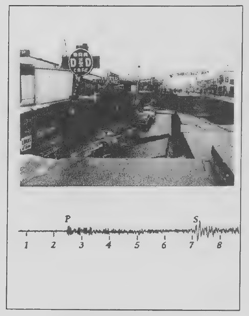Transparency 12-1-1

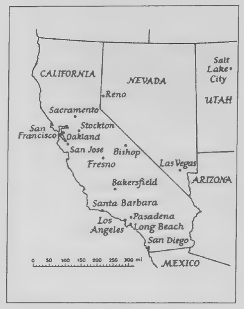Transparency 12-1-2

Chapter 12: Circles

Lesson 1: Circles, Radii, and Chords

Lesson Outline

Terms: Circle, concentric, radius, chord, diameter. Corollary to the Definition of a Circle. All radii of a circle are equal. Theorem 56. If a line through the center of a circle is perpendicular to a chord, it also bisects the chord. Theorem 57. If a line through the center of a circle bisects a chord that is not a diameter, it is also perpendicular to the chord. Theorem 58. The perpendicular bisector of a chord of a circle contains the center of the circle.

Transparencies

12-1-1_ Photograph of Anchorage earthquake 12-1-2. Map: California

Introduction

The photograph on Transparency 12-1-1 was taken in downtown Anchorage, Alaska, after an earthquake in 1964. The street in the picture was not very far from the earthquake’s epicenter, or point of origin.

Scientists are now able to locate the epicenter of an earthquake quite accurately, even though it may be hundreds of miles from any populated area. When an earthquake occurs, its vibrations are recorded by seismographs. The graph on Transparency 12-1-1 was made on a rotating drum ina seis-

mograph and shows the shock waves of an earthquake. The vertical segments mark off minutes. A little after two minutes from the beginning of the hour, the primary, or P, wave appeared; about five minutes later, it was followed by a secondary, or S, wave. By measuring the time interval between these two waves, seismologists can determine the distance the waves traveled and, hence, how far away the epicenter is.

Hand out duplicated copies of Transparency 12-1-2. Suppose that the waves of an earthquake are picked up by a seismograph at Cal Tech in Pasadena and that they show the epicenter is 230 miles away. Where could the epicenter be? (Somewhere on a circle with a radius of 230 miles and Pasadena as its center.) Have your students set their compasses to this radius, using the scale at the bottom of the map, and draw the circle. Suppose that a seismograph at the University of California at Berkeley, on the other hand, shows that it is 210 miles away from the epicenter of the same earthquake. Draw a second circle having this radius and with its center just above Oakland. What does this tell us about the location of the epicenter? (It could be in one of two places.) Suppose that the University of Nevada at Reno reports that the earthquake is 170 miles away. Draw a circle to illustrate this. What can you conclude from the three circles? (That the epicenter is the point in which they intersect, near Bishop, California.)

Transparency 12-2-1: Plane-perspective problem

Transparency 12-2-2: Plane-perspective solution

Transparency 12-3-1: “The Theory of the Rainbow”

After remarking that the circle is of great importance in geometry, both because of its many interesting properties and because of its wide variety of practical applications, you might either present the lesson as in the text or assign it for individual study.

Lesson 2: Tangents

Lesson Outline

Terms: Tangent line.

Theorem 59. If a line is tangent to a circle, it is perpendicular to the radius drawn to the point of contact.

Theorem 60. If a line is perpendicular to a radius at its outer endpoint, it is tangent to the circle.

Transparencies

• 12-2-1 Plane-perspective problem
• 12-2-2 Plane-perspective solution

Introduction

The problem on Transparency 12-2-1 appears in an issue of the in-flight magazine published by Delta Airlines. Help your students draw a figure to illustrate it, introducing the term tangent as you do so. As you draw the radius to the point of contact, ask how it seems to be related to the tangent. Explain that this can be proved, so that it is correct to assume that the triangle with its vertices at the airplane, the horizon point, and the center of the earth is a right triangle.

In discussing the solution, it is worth noting that the answer can be estimated without a calculator by factoring rather than squaring:

d = (4,005)? — (4,000)?

— (4,005 + 4,000)(4,005 — 4,000)

= +(8,005)(5) = 440,000

= 200. The horizon appears about 200 miles away.

After finding the solution, your students will be interested in seeing Transparency 12-2-2, on which the answer given in the airline magazine appears. Obviously only passengers who had taken geometry would have been able to solve this problem—or even understand the solution given.

Remind your students that, in finding the solution, we assumed that the tangent is perpendicular to the radius drawn to the point of contact. This proof of this theorem and its converse can then be presented as in the text.

Lesson 3: Central Angles and Arcs

Lesson Outline

Terms: Semicircle, minor arc, major arc, central angle, reflex angle, degree measure of an arc.

Postulate 10. The Arc Addition Postulate. If C is on AB, then mAC + mCB = mACB.

Theorem 61. Ina circle, equal chords have equal arcs.

Theorem 62. In a circle, equal arcs have equal chords.

Transparencies

• 12-3-1 “The Theory of the Rainbow”
• 12-3-2 Photograph of rainbow

Transparency 12-3-2: Photograph of rainbow

Transparency 12-4-1: Longest field goal

Transparency 12-4-2: Football field diagram

Introduction

The Greek philosopher Aristotle is thought to have been the first person to try to explain the rainbow. A lengthy article about the modern theory of the rainbow appeared in the April 1977 issue of Scientific American; the first page of this article is reproduced on Transparency 12-3-1. It, together with the rainbow photograph that appears on Transparency 12-3-2, would make a nice introduction to the new lesson. The lesson can then be presented as in the text.

Lesson 4: Inscribed Angles

Lesson Outline

Terms: Inscribed angle.

Theorem 63. An inscribed angle is equal in measure to half its intercepted arc.

Corollary 1. Inscribed angles that intercept the same arc are equal.

Corollary 2. An angle inscribed in a semicircle is a right angle.

Transparencies

• 12-4-1 Longest field goal
• 12-4-2 Football field diagram

Introduction

The longest field goal in professional football was kicked by Tom Dempsey in a game between the New Orleans Saints and the Detroit Lions in 1970. The kick, shown on Transparency 12-4-1, covered a distance of 63 yards and is especially amazing because Dempsey has had only half a right foot since birth.

Mark a point on Transparency 12-4-2 to represent a spot 53 yards from the upper goal line (the distance from the goal line to the goal post is 10 yards) and draw rays from that point to the lower corners of the goal post. To make the goal, Dempsey had to kick the ball within this angle, which has a measurte of less than 6°! At what other spots on the field would the angle be the same? Explain that the answer to this question comes from a theorem of the new lesson and present the rest of the lesson as in the text. After the lesson has been completed, show Transparency 12-4-2 again. Explain that the other points on the field for which the goal post angle is the same lie on a circle that contains the kicking point and the corners of the goal post. We know that the angles are equal because of the corollary that inscribe angles that intercept the same arc are equal.

Lesson 5: Secant Angles

Lesson Outline

Terms: Secant, secant angle.

Theorem 64. A secant angle whose vertex is inside a circle is equal in measure to half the sum of the arcs intercepted by it and its vertical angles.

Theorem 65. A secant angle whose vertex is outside a circle is equal in measure to half the difference of its larger and smaller intercepted arcs.

Transparencies

• 12-5-1 Cinerama projector system

Transparency 12-5-1: Cinerama projector system

Transparency 12-6-1: Galileo and the moon

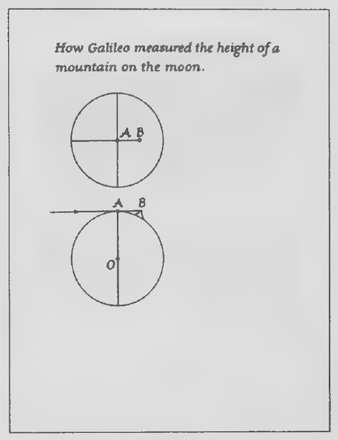Transparency 12-6-2: How Galileo measured the height of a mountain on the moon

Introduction

In the 1950s, a motion-picture process using three projectors and a curved screen was introduced. Called “Cinerama,” this process produced a stronger sense of reality than the ordinary flat screen, but it was so expensive to operate that it was given up in the 1960s.

The figure on Transparency 12-5-1 is an overhead view of a Cinerama auditorium, showing the screen and projectors. Add Overlay A and explain that the circle has been divided into 10° arcs. Each projector, then, covers 40° of the screen. Place Overlay B so that the vertex of the projector angle falls on the center of the circle. From the intercepted arc, we see that the projector angle has a measure of 30°. Now, place Overlay B in positions to illustrate an inscribed angle and a secant angle whose vertex is inside a circle. Overlay C can be used to illustrate secant angles whose vertices are outside a circle. After your students have discovered the measure relations between secant angles whose vertices are inside and outside a circle and their intercepted aracs, the proofs of the two secant angle theorems can be developed as in the text.

Lesson 6: Tangent Segments and Intersecting Chords

Lesson Outline

Terms: Tangent segment.

Theorem 66. The Tangent Segments Theorem. The tangent segments to a circle from an external point are equal.

Theorem 67. The Intersecting Chords Theorem. If

two chords intersect in a circle, the product of

the lengths of the segments of one chord is

equal to the product of the lengths of the

segments of the other chord.

Transparencies

• 12-6-1 Galileo and the moon
• 12-6-2 How Galileo measured the height of a

mountain on the moon

Introduction

Before Galileo first looked at the night sky through his telescope in the fall of 1609, it was generally believed that the surface of the moon, unlike that of the earth, was perfectly smooth. Galileo noticed that the boundary between the dark and light sides of the moon was very ragged and concluded from this observation that the moon must have mountains and valleys. He made the painting of the moon shown on Transparency 12-6-1 from observations made through his telescope.

Notice that there are several light spots on the dark side, not far from the boundary of the lighted side. Galileo figured that these spots must be mountain peaks high enough to catch some light from the rising or setting sun. With this as the basis of his reasoning, he used some simple geometry to measure the height of a mountain on the moon.

Hand out duplicated copies of Transparency 12-6-2. The first figure represents the moon and one of the light spots, at B, as seen through Galileo’s telescope. The second figure represents a “side view” of the same thing: a ray of light from the sun is tangent to the moon at A and hits the top of the mountain peak at B. Galileo estimated the distance from

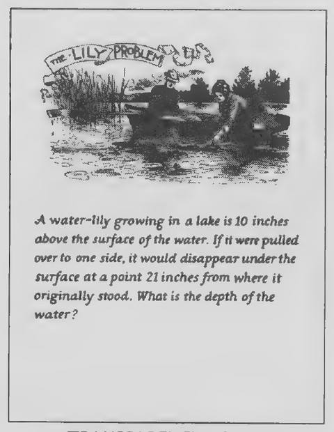Transparency 12-R-1

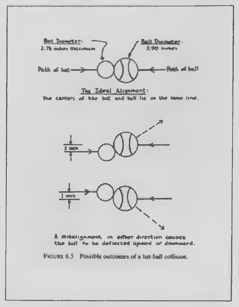Transparency 12-R-2: Baseball misalignment

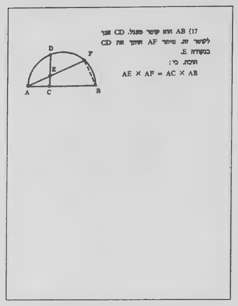Transparency 12-R-3: A proof from a Hebrew geometry book

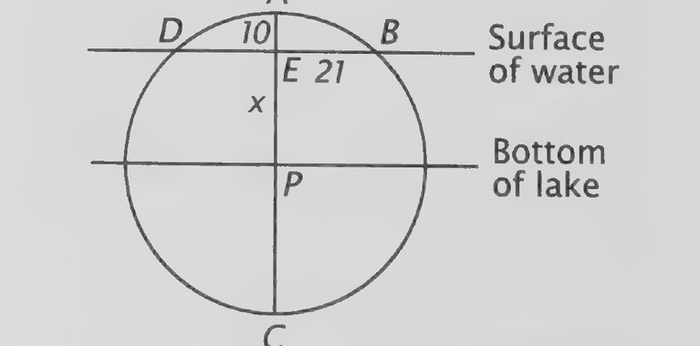Figure on page 378 — A circle cut by chords and a segment of length 10, with the unknown length x marked

A to B by comparing it with the radius of the moon.

In these figures, AB appears to be about 5 the length

of the radius; but in his painting, Galileo figured

that AB was about — as long as the radius.

12

Galileo knew that the radius of the moon was

1 1,080 miles, and so he estimated AB as 7p (1,080) =

90 miles. Write the lengths of OA and AB on the second figure, draw OB, and give your students some time to figure out the height of the mountain at B.

Because AB is tangent to the circle at A, AB LOA, and so △AOB is a right triangle. Applying the Pythagorean Theorem,

OB? = 1,0802 + 902 = 1,174,500 And so

OB = 1,174,500 = 1083.7. Therefore, the mountain at B is about 3.7 miles high.

Review of Chapter 12

Transparencies

12-R-1_ Longfellow’s water-lily problem 12-R-2 Baseball misalignment 12-R-3 A proof from a Hebrew geometry book

First day

Introduction

The most popular American poet of the nineteenth century was Henry Wadsworth Longfellow. Longfellow was also an amateur mathematician and

among the problems that he created was one about a water lily in a lake.* (Show Transparency 12-R-1 with the overlay in place.)

A water lily growing in a lake is 10 inches above the surface of the water. If it were pulled over to one side, it would disappear under the surface at a point 21 inches from where it originally stood. What is the depth of the water?

To solve this problem, we need a diagram. Remove the overlay and guide your students in drawing the figure shown below. First, draw just the two horizontal lines and PA. As the water lily is pulled over to one side, what kind of path does the top of it follow? Draw AB and then the entire circle; also, draw the entire diameter AC.

A

Surface

of water

Bottom

of lake

‘This problem was originally in Sam Loyd’s Cyclopedia of Puzzles, privately published in 1914. It is included in Mathematical Puzzles of Sam Loyd, volume 1, selected and edited by Martin Gardner (Dover, 1959).

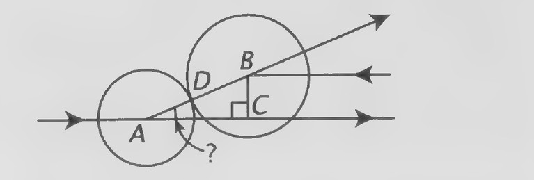Figure on page 379 — Two circles tangent to a common line and to each other’s external tangents (points A–D marked)

Label EA, EB, and EP as indicated. Then ask your students how they would label ED and PC. (We are assuming that the water lily is originally perpendicular to the surface of the water so that AC bisects DB. ED = 21 and PC = x + 10.) Point out that, without adding anything more to the figure, the Intersecting Chords Theorem can be used to solve for x. Let a student demonstrate his or her solution to the class. Because DE · EB = AE · EC, 21² = 10(2x + 10). Solving for x, x = 17.05. The lengths in the problem are each given as a whole number of inches, and so it is appropriate to round this answer and to say simply that the lake is about 17 inches deep.

Second day

Introduction

The figures on Transparency 12-R-2, which show some possible outcomes when a baseball is struck by a bat, are from Sport Science by Peter J. Brancazio (Simon & Schuster, 1984). The first figure illustrates the ideal situation, in which the bat hits the ball head-on with the greatest possible force. The other figures show situations in which the bat and ball are not perfectly aligned so that the ball is popped up or hit toward the ground.

Have your students draw and label the second figure as shown at the right. On the assumption that the paths of the bat and ball are parallel and a misalignment of 1 inch, at what angle with the path of the bat is the ball deflected? In making the calculation, use the diameters of the bat (2.75 in) and ball (2.90 in) given.

In right △ABC,

BC = 1 and AB = (2.75 + 2.90)/2 = 2.825.

By the definition of the sine ratio,

sin A = BC/AB = 1/2.825 ≈ 0.354

And so ∠A ≈ 21°. The ball is deflected at an angle of approximately 21°.

The proof exercise on Transparency 12-R-3, taken from a Hebrew geometry book, might be used for further review. The “given” seems to be that AB is a diameter of the circle of which the arc is a part, that CD ⊥ AB, and that AF intersects CD at E. FB is evidently an auxiliary line, added as a clue to the proof. The proof is based on showing that the two triangles in the figure are similar.

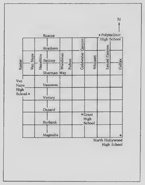Transparency 13-1-1: Locations of schools

Transparency 13-2-1: Oak Island in the news

Chapter 13: The Concurrence Theorems

Lesson 1: Triangles and Circles

Lesson Outline

Terms: Cyclic, circumcircle, circumcenter, polygon inscribed in a circle, circle circumscribed about a polygon. Theorem 68. Every triangle is cyclic.

Corollary. The perpendicular bisectors of the sides of a triangle are concurrent.

Construction 9. To circumscribe a circle about a triangle.

Transparencies

• 13-1-1 Locations of schools

Introduction

The following problem provides a nice introduction to the ideas of Lesson 1. I will describe it exactly as I present it to my own class; if it is not possible to recast the problem in terms of your own neighboring schools, you might state it in terms of fire stations or some other local landmarks.

Before Grant opened in 1959, the three high schools in this area were North Hollywood High, Van Nuys High, and Polytechnic High. Hand out a map comparable to the one on Transparency 13-1-1 to each student. This map shows the locations of these schools and of Grant. For simplicity, each school has been represented by a single point. As you can see, Grant is closer to North Hollywood High than to the other two schools. It might have

been better to have located Grant so that its distances to the three schools were the same. For convenience, we will refer to the points representing the schools by the first letters of their names. Guess, without doing any measuring, where you think the point that is equidistant from V, P, and N is located and mark it with a small x.

If the point that you have guessed is really equidistant from V, P, and N, it should be possible to draw a circle with it as center that passes through all three points. See if you can do this.

Can you think of a way to use your straightedge and compass to find the point equidistant from V, P, and N that does not involve any guessing? (If necessary, ask where the points that are equidistant from just two of these points are located.) After someone has suggested constructing the perpendicular bisectors of the segments joining the points, have your students draw △VPN and construct the perpendicular bisectors of two of its sides.

How close is the point in which the two lines intersect to the point you marked x? Try to draw a circle with the point in which the two lines intersect that passes through all three vertices of the triangle.

Explain that △VPN is called “cyclic.” The rest of the lesson can be developed as in the text.

Transparency 13-2-2: Navigation chart

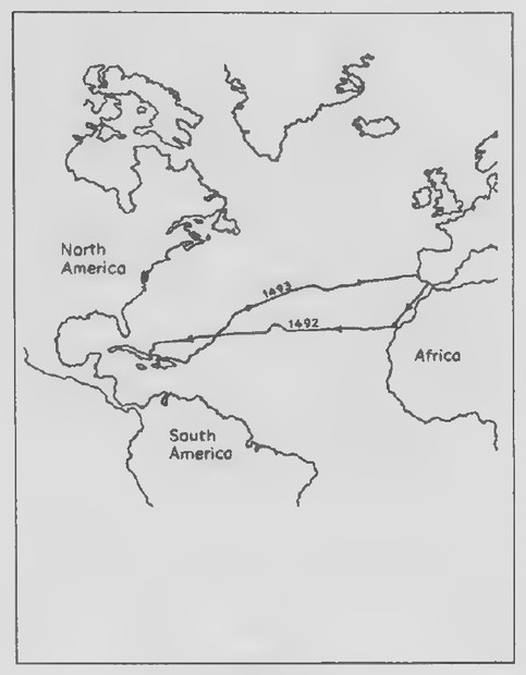Transparency 13-3-1: Map: Voyage of Columbus

Transparency 13-3-2

Lesson 2: Cyclic Quadrilaterals

Lesson Outline

Theorem 69. A quadrilateral is cyclic iff a pair of its opposite angles are supplementary.

Transparencies

• 13-2-1 Oak Island in the news
• 13-2-2 Map: Oak Island

Introduction

Ever since 1795, people have been searching for buried treasure on a small island off the coast of Nova Scotia. The island, named Oak Island, is pictured on Transparency 13-2-1. It has been speculated that as much as $30 million worth of treasure may be buried on the island, perhaps by Blackbeard the Pirate or Captain Kidd.

There is an elaborate maze of tunnels below the island’s surface, which engineers say must have taken several years to construct. Unfortunately for people looking for the treasure, these tunnels seem to have been designed to flood any holes that may be dug on the island. Even though little evidence of buried treasure has been discovered, the tunnel system may very well have been built to protect it from discovery.

Hand out duplicated copies of Transparency 13-2-2. This map shows the part of Oak Island where the treasure is thought to be buried. Can you find the exact spot, given that it is equidistant from the four lettered points on the map?

After your students have found the spot, observe that any three of the four lettered points are sufficient to locate it. Draw the circle that contains

all four points and the quadrilateral having those points as its vertices. Observe that this quadrilateral is cyclic because its vertices lie on a circle. After pointing out that, unlike triangles, not every quadrilateral is cyclic, present the rest of the lesson as in the text.

Lesson 3: Incircles

Lesson Outline

Terms: Circle inscribed in a polygon, polygon circumscribed about a circle, incircle, incenter.

Theorem 70. Every triangle has an incircle.

Corollary. The angle bisectors of a triangle are concurrent.

Construction 10. To inscribe a circle in a triangle.

Transparencies

• 13-3-1 Map: Voyage of Columbus
• 13-2-2 Navigation chart

Introduction

The map on Transparency 13-3-1 shows the paths of Columbus’s ships in his historic voyage from Spain to the New World and back again. Although pilots of modern ships have several methods for determining their positions at sea, Columbus used celestial navigation. He kept track of where he was by observing the sun and moon, the planets, and the stars.

A navigator records each sighting as a line on a chart. Three lines are usually used, and, if there are no inaccuracies, they intersect in a point that is the ship’s position. Hand out duplicated copies of Transparency 13-3-2. This figure shows what usually hap-

Transparency 13-4-1: A problem of gravity

pens: the three lines do not intersect in a common point, but form a triangle. The navigator takes the point that is equidistant from the sides of the triangle as the position of the ship. According to the standard reference on navigation, this point “can be determined geometrically or by computation, but in normal practice the navigator estimates it by eye.”* a Have your students estimate the point that is equidistant from the sides of the triangle by eye. Remark that if the point is correct, it should be possible to draw a circle with this point as center that is tangent to each side of the triangle. A discussion of how to do this leads into the rest of the ideas of the lesson.

Lesson 4: The Centroid of a Triangle

Lesson Outline

Terms: Median, centroid, orthocenter.

Theorem 71. The medians of a triangle are concurrent.

Theorem 72. The lines containing the altitudes of a triangle are concurrent.

Transparencies

13-4-1_ A problem of gravity

Introduction

Give each student an unlined 4-in x 6-in file card and a pair of scissors. Have your students mark the point on the upper edge 2 inches from the left cor-

ner as shown on Transparency 13-4-1 and draw lines from this point to the lower left and right corners of the card. Cut along these lines and put the two smaller pieces aside.

It is easy to balance the largest triangular piece on three fingers so that it is horizontal. (Illustrate this and have everyone do it.) It is not as easy to balance it on just two fingers. Can you do it? Can you balance the “triangle” on just one finger? (After a few attempts, most students should be able to do this.) Now a very challenging question. Can you balance the “triangle” on the metal point of your compass? You may poke a small hole in the card at whatever point you think will work. (It is unlikely that anyone will be able to guess the precise point on which the triangle may be balanced.)

Let’s see if we can find the balancing point by construction. Make a careful tracing of the triangular piece on a sheet of paper. What lines do you think we should draw in order to find the balancing point? (Have everyone try out any suggestions made. Someone will probably guess that the triangle will balance on its circumcenter and someone else its incenter. When each of these points has been located, it should be labeled on the card. After discovering that neither point will work, someone may think of the triangle’s altitudes. If so, construct them, and, after the class has observed that they seem to be concurrent, label the point as the orthocenter. Because the idea of a median ina triangle has not been considered previously in the course, no one may think of drawing the medians. If this is the case, you might give the following clues.)

It seems that, if the triangle is to balance on one

*Dutton’s Navigation and Piloting, 14th edition, by Elbert S. Maloney (Naval Institute Press, 1985), page 417.

Transparency 13-5-1: Cartoon of geometers and triangle

Transparency 13-5-2: Encyclopedia Britannica article on Ceva

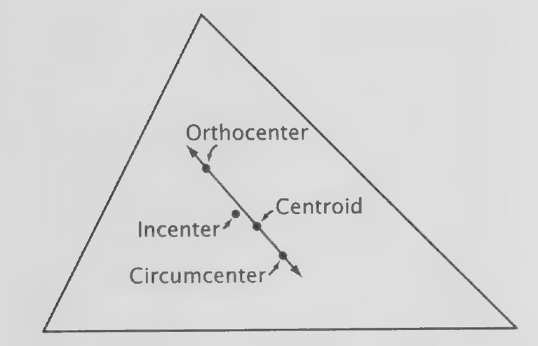Figure on page 383 — A triangle with its orthocenter, incenter, centroid, and circumcenter marked

and half on the other. In other words, each of the line determining this point should divide the triangle in half. Where do you suppose a line from one vertex of the triangle should be drawn in order to divide the triangle in half? (To the midpoint of the opposite side.) After everyone has drawn the medians, observe that they also seem to be concurrent and then let everyone see if the triangle will

ce: balance on this point.

Proofs that the medians of oe triangle neon current and that the lines containing the altitudes are concurrent are considered in the exercises of the

lesson.

Lesson 5: Ceva’s Theorem

Lesson Outline

Terms: Cevian.

Theorem 73. Ceva’s Theorem. Three cevians, AY, BZ, and CX, of △ABC are concurrent iff

Transparencies. 13-5-1 Cartoon of geometers and triangle 13-5-2 Encyclopedia Britannica article on Ceva

Introduction

The cartoon on Transparency 13-5-1 was drawn by Kenneth J. Neal when he was a student at Penn Hills High School in Pittsburgh. It illustrates an imaginary discussion of the triangle between a Greek mathematician—perhaps Euclid or Pythagoras—and some European mathematicians of the seventeenth century. One of these mathematicians might be Ceva, whose theorem is the subject of the new lesson. Before introducing the theorem and its proof, show Transparency 13-5-2, on which the article on Ceva in the micropedia section of the Encyclopedia Britannica is reproduced. I recommend having your students draw the figures and write the key equations in the proof that if the cevians are concurrent, the product of the ratios is equal to one. The proof

of the converse is probably best left to be read as part of the assignment.

Transparency 13-6-1: Something old and something new

Transparency 13-6-2: Encyclopedia Britannica article on Morley’s

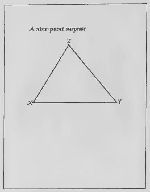Transparency 13-R-1: A nine-point surprise

Lesson 6: Napoleon’s Discovery and Other Surprises

Lesson Outline

Transparencies

• 13-6-1 Something old and something new
• 13-6-2 Encyclopedia Britannica article on Morley’s

Theorem

Introduction

Hand out duplicated copies of Transparency 13-6-1. If the calendar were suddenly turned back 2,000 years and you were still a high school (or college) student, you wouldn’t be taking some of the courses that you take now because they wouldn’t exist. Other courses that you are taking would probably be radically different from what they are now. Much of geometry, however, would be very much the same.

For example, the fact that the angle bisectors of every triangle are concurrent is established in Euclid’s Elements. Use your straightedge and compass to construct, as accurately as you can, the angle bisectors of the first triangle on the sheet you have been given. After your students have done this, have them label the figure “The angle bisectors of a triangle are concurrent—proved by Euclid c. 300 B.C.”

What would happen if, instead of bisecting the angles of a triangle, we trisected them? You may recall that it is impossible to trisect most angles with: just a straightedge and compass. Because this is the case, we will use a protractor instead. Give your students time to draw the trisectors of the three angles as accurately as they can. To make this easier, the triangle has been drawn so that the measures of its

angles are 30°, 51°, and 99°. Demonstrate the procedure on the overhead projector. If the three points of intersection of the adjacent trisectors of the angles are connected with line segments, an equilateral triangle is formed!

This is a relatively new theorem in elementary geometry because it was discovered at the end of the nineteenth century. Label the figure “The angle trisectors of a triangle determine the vertices of an equilateral triangle—discovered by Frank Morley in 1899.” Frank Morley was a professor of mathematics at Johns Hopkins University and the father of the author Christopher Morley. It was not until ten years after Morley made this discovery that someone figured out how to prove it. The entry on Morley’s Theorem in the Encyclopaedia Britannica is on Transparency 13-6-2. A proof of the theorem can be found in Geometry Revisited by H. S. M. Coxeter and S. L. Greitzer, a book in the New Mathematical Library (M.A.A., 1967) but it is by no means easy.

Review of Chapter 13

Transparencies

• 13-R-1 A nine-point surprise
• 13-R-2 Review: The spotter’s puzzle

First day

Introduction

Hand out duplicated copies of Transparency 13-R-1. The following directions are for a rather elaborate construction that provides a good review of ideas as well as having an interesting result. First, construct the three altitudes of the triangle and name them XE, YG, and ∠A. Label the orthocenter of the

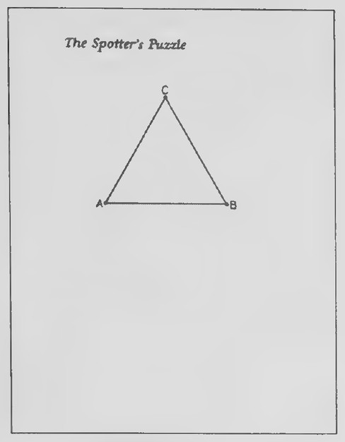Transparency 13-R-2: Review: The spotter’s puzzle

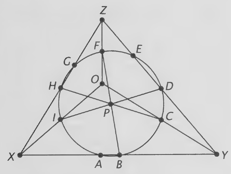Figure on page 385 — A triangle with an inscribed circle, a circumscribed circle, and the Euler line through its centers

Next, bisect the three line segments connecting the orthocenter of the vertices of the triangle. Label their midpoints as follows: OX, midpoint I; OY, midpoint C; OZ, midpoint F.

Next, find the midpoints of the sides of the triangle and label them as follows: XY, midpoint B; YZ, midpoint D; XZ, midpoint H.

What do you notice? (The points labeled A through I appear to lie on a circle.) That the nine points we have labeled A through I should lie on a circle is quite remarkable. It is not difficult to find the center of the circle because six of them are the endpoints of three of the circle’s diameters. Can you guess which points these are? (The three diameters are FB, HC, and ID.) Draw the three diameters, label the point in which they are concurrent P, and draw the “nine-point” circle.

Two interesting properties of the “nine-point” circle are that its center is the midpoint of the line segment connecting the orthocenter and the circumcenter of the triangle and that its radius is half the radius of the circumcircle of the triangle.

Some of your better students might be interested in seeing a proof of why the nine points lie on a circle. An especially straightforward one is in Excursions in Geometry by C. Stanley Ogilvy (Oxford University Press, 1969), pages 119-120. Historians are not sure who first noticed the “nine-point” circle. The first proof of its existence seems to have been published in 1821.

Second day

Introduction

This is an appropriate point at which to reconsider the spotter’s puzzle introduced at the beginning of the course. Begin by showing Transparency 0-4 and recalling the story of the surfer and the spotter. Your students may have already proved that it doesn’t matter where the surfer builds his house on the island: the sum of the lengths of the perpendicular segments to the sides from every point on the island is the same.*

For the spotter, who wanted to build his house so that the sum of the lengths of the paths from it to the three corners of the island is aminimum, the situation is quite different. The sum depends on the position of the point. Show your students Transparency 0-5 and its overlay to remind them that the sum seems to be the smallest at the “center” of the

*See Chapter 9, Lesson 3, exercises 29-34, on page 355.

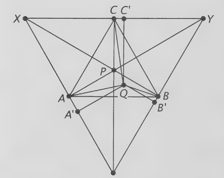Figure on page 386 — Two similar right triangles sharing a vertex, with the perpendicular segments that give the proportions marked

triangle.

Hand out duplicated copies of Transparency 13-R-2 and ask how the “center” of the triangle can be found. Using congruent triangles, it is easy to show that the angle bisectors, altitudes, medians, and hence, the perpendicular bisectors of the sides, of an equilateral triangle are all the same. So the four centers of the triangle that are determined by these lines are the same point. Find the point and label it P. Notice that ∠APB = ∠BPC = ∠CPA = 120° because the six small triangles formed by the lines are 30°-60° right triangles.

(Ss

BN

A

Next, choose any other point in the triangle, label it Q, and draw QA, QB, and QC. We will show that PA + PB + PC is less than QA + QB + QC and thus prove that the sum of the lengths of the paths from point P to the three vertices is less than the sum from any other point, such as Q.

To do this, we draw lines through the vertices of △ABC so that they are perpendicular to PA, PB, and PC. Label the triangle formed by these lines

△XYZ as shown in the figure above. Looking at quadrilateral XAPC, we see that ∠XAP = 90°, ∠APC = 120°, and ∠PCX = 90°, and so ∠CXA = 60°. By the same reasoning, we can conclude that the other two angles of △XYZ also have measures of 60°, and so △XYZ is equiangular and hence equilateral.

Now draw perpendicular segments from to the sides of △XYZ and label them as shown. Notice that QA’ < QA, QB’ < QB, and QC’ < QC because the perpendicular segment from a point to a line is the shortest segment connecting them.

Finally, observe that we have shown △XYZ to be equilateral and recall that, in reviewing the surfer’s puzzle, we proved that for an equilateral triangle, the sum of the lengths of the perpendicu-

lar segments to the sides from every point in the triangle is the same. Therefore,

PA + PB + PC = QA’ + QB’ + QC’. We have shown that QA’ < QA, QB’ < QB, and @Cy—OG 750

QA’ + OB’ + OC’ =QA + QB + QC, and hence,

PA + PB + PC <QA+ QOB+ QC.

This proof that P is the minimum point was invented by Evangelista Torricelli, an Italian mathematician who also invented the barometer. If the original triangle is not equilateral, then point P is not the circumcenter, incenter, orthocenter, or centroid, but a fifth point called the “Fermat point.” This point is named for Pierre Fermat, who first proposed the general version of the spotter’s problem in the seventeenth century. It is the point such that the segments joining it to the vertices of the triangle form equal angles of 120°.

More information on Fermat’s problem can be found in Mathematical Gems I by Ross Honsberger (M.A.A., 1973), pages 24-34.

Transparency 14-1-1: Photograph of water-bug egg

Transparency 14-1-2: Cyclic polygon figure

Transparency 14-2-1: Picture of Gauss

Chapter 14: Regular Polygons and the Circle

Lesson 1: Regular Polygons

Lesson Outline

Terms: Regular polygon, center, radius, central angle, apothem. Theorem 74. Every regular polygon is cyclic.

Transparencies

• 14-1-1 Photograph of water-bug egg
• 14-1-2 Cyclic polygon figure

Introduction

The photograph on Transparency 14-1-1 was taken through an electron microscope by an entomologist. (A student who is familiar with the word might explain its meaning: a person who studies insects.) The photograph shows the surface of one of the eggs of a water bug. The extreme magnification (820x) reveals that the surface is covered with an elaborate network: this network seems to consist of polygons of various shapes. In what basic way are all of the polygons alike? (They are all convex.)

Add the overlay to the transparency and ask your students to identify the three polygons shown by name. The hexagon seems to be more symmetric than the other two. Why? (Because its sides and angles are close to being equal.) A convex polygon that is both equilateral and equiangular is called regular.

Following this introduction, hand out duplicated copies of Transparency 14-1-2 and use them

to develop the proof that every regular polygon is cyclic. The figure shows only part of a regular polygon to emphasize that the proof is independent of the number of sides.

Lesson 2: The Perimeter of a Regular Polygon

Lesson Outline

Theorem 75. The perimeter of a regular polygon

having n sides is 2Nr, in which N =n sin a and r is its radius.

Transparencies

• 14-2-1 Picture of Gauss
• 14-2-2 Regular polygon constructions
• 14-2-3 Construction of a regular 17-gon
• 14-2-4 A regular pentagon

Introduction

Carl Friedrich Gauss, whose picture is on Transparency 14-2-1, was born in 1777 and died in 1855. Now considered one of the greatest mathematicians of all time, Gauss made an interesting discovery about regular polygons when he was nineteen years old.

Show Transparency 14-2-2. In yesterday’s lesson, we proved that every regular polygon is cyclic. Constructing a regular polygon with a given number of sides is equivalent to being able to locate that number of equally spaced points on a circle. Add the overlay to Transparency 14-2-2. Euclid be-

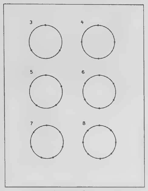Transparency 14-2-2: Regular polygon constructions

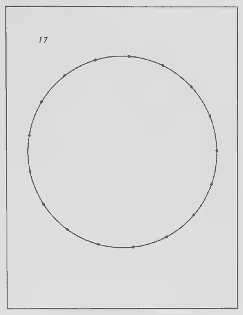Transparency 14-2-3: Construction of a regular 17-gon

Transparency 14-2-4: A regular pentagon

gan the Elements with an explanation of how to construct the simplest of the regular polygons—the equilateral triangle. Later he showed how to construct several other regular polygons by inscribing them in circles. These include the square, regular pentagon, and regular hexagon. By bisecting their central angles, other regular polygons having twice as many sides can be constructed.

Notice that the regular heptagon is missing. Euclid omitted it from the Elements, and for more than two thousand years it was unclear as to whether it is possible to construct a regular heptagon with just a straightedge and compass. Finally, in 1796, Gauss proved that the construction is impossible.

Show Transparency 14-2-3. At the same time that Gauss proved that seven equally spaced points cannot be located on a circle with just a straightedge and compass, he made a surprising discovery: it is possible to locate seventeen evenly spaced points using these tools. The method for doing so, as you might imagine, is quite complicated. (Add the overlay to Transparency 14-2-3.) Through a long series of steps, the vertical segments at the left and right are drawn. These segments cut off an arc of the circle that is exactly two-seventeenths of it. This arc is then divided in half to produce an arc that is exactly oneseventeenth of the circle. The method is described, together with a brief history of the constructability of the regular polygons, in Introduction to Geometry, Second Edition, by H. S. M. Coxeter (Wiley, 1969), pages 26-28.

To use in deriving the equation for the perimeter of a regular polygon in terms of its radius, I

recommend providing your students with duplicated copies of Transparency 14-2-4. (Having a large, accurate figure to work with is important and this saves time that would be needed by your students to try to draw one.)

Lesson 3: The Area of a Regular Polygon

Lesson Outline

Theorem 76. The area of a regular polygon having n sides is Mr², in which M = ½n·sin(360°/n) and r is its radius.

Transparencies

• 14-3-1 Octagon Spa advertisement
• 14-3-2 Regular octagon

Introduction

The advertisement for the octagonal spa that is reproduced on Transparency 14-3-1 raises the question of how the area of a regular polygon might be determined. Explain that the central objective of this lesson is to derive an equation for the area of a regular polygon in terms of its radius and hand out duplicated copies of Transparency 14-3-2 for use in doing this.

After you have the equation, return to the octagon advertisement and show how its area can be determined. The dimension of the octagon given is its longest dimension: that is, the distance from a vertex to the opposite vertex. The radius of the octagon, then, is 3.5 feet. Guide your students in using their calculators to find its area. (It is approximately 34.7 square feet.)

Transparency 14-3-1: Octagon Spa advertisement

Transparency 14-3-2: Regular octagon

Transparency 14-4-1: Russian dolls in a row

Lesson 4: From Polygons to Pi

Lesson Outline

Terms: Circumference, limit, pi. Theorem 77. If the radius of a circle is r, its circumference is 2mr. Corollary. If the diameter of a circle is d, its circumference is Td.

Transparencies

• 14-4-1 Russian dolls in a row
• 14-4-2 Russian dolls in a stack

Introduction

Anice way to introduce the idea of a limit is to show a set of Russian Matreshka dolls. The dolls are wooden and nest inside each other to represent a sequence of generations. The set that I use consists of twelve dolls ranging in height from almost 20 cm to less than 1 cm. If you have such a set, your students will enjoy seeing the actual dolls. If not, the picture on Transparency 14-4-1 shows what they look like.

Each successive doll is about 75% as tell as the one before it. Suppose that there were no end to the smaller dolls and that this size ratio continued. To what number do you think the heights of the successive dolls would get closer and closer? Even though we would never come to a doll whose height is actually zero, we say that the heights of the dolls approach zero as a limit.

Show Transparency 14-4-2, keeping the table covered. Now suppose that, as we come to each successive doll, we stack them one on top of another. Do you think that we could make the stack as tall as

we please? For example, do you think if we had enough dolls, we could make a stack a mile high?

Show the table on Transparency 14-4-2 and explain that the first column represents the numbers of the dolls, the second column their heights, and the third column the heights of the stacks as more and more dolls are added. Beginning with the fifth line, the numbers have been rounded to four decimal places. After the tenth doll, the table jumps ahead to lines later in the sequence. What number does the height of the 100th doll seem very close to? What number does the height of the stack of the first 100 dolls seem very close to? If even more dolls were added to the stack, the height would continue to get closer and closer to 80 cm. For this reason, we say that it approaches 80 as a limit.

Following this introduction, the lesson on the circumference of a circle as the limit of the perimeters of the inscribed regular polygons can be presented as in the text.

Lesson 5: The Area of a Circle

Lesson Outline

Terms: Area of a circle.

Theorem 78. If the radius of a circle is 1, its area is πr².

Transparencies

• 14-5-1 Digits of pi

Introduction

Before class, I stretch adding machine tape on which I have written the value of 7 to several hundred decimal places across the front, a side, and back

Transparency 14-4-2: Russian dolls in a stack

Transparency 14-5-1: Digits of pi

Transparency 14-6-1: Photograph of the Indianapolis Speedway

walls of my classroom. A table listing 1,650 decimal places of mis given on Transparency 14-5-1. I found a spacing of 2 inches per digit convenient. In lieu of the tape, you might, of course, simply show Transparency 14-5-1.

The history of tis very interesting. If you have a copy of the book A History of m by Petr Beckman (Golem Press, 1971), I recommend showing it to your class and then telling your students some of the story. The following outline lists some of the major events.

Tl Decimal Places 2000 B.C. Babylonians: 3 1/8 1 300 B.C. Euclid: 3.14 Z 1504.D. Ptolemy: 3.1416 4 1610 Van Ceulen $10)

Calculus invented in 17th century

1706* Machin 100 1873 William Shanks 707, but wrong after 526

Computers invented in 20th century

1949 ENIAC 2,000 1959 IBM 704 (Paris) >10,000 1961 IBM 7090 (New York) 100,000 1973 (Paris) 1,000,000 1981 (New York) 1,000,000,000 2002 (Tokyo) >1,000,000,000,000

Before the discovery of calculus, approximations of m were obtained from regular polygons. Ludolph van Ceulen, a sixteenth-century Dutch

professor of mathematics and military science, carried out his calculation of 7 to 35 decimal places by starting with a regular polygon having 60 sides and doubling 29 times to get a polygon having more than 32 billion sides!

One of my students once learned the value of 7 to 50 decimal places, but according to the Guinness Book of World Records, in 1981 a 23-year-old man in India recited 31,811 places of m from memory, part of which was broadcast over the radio. It took him more than three hours, going at a rate of more than 150 digits per minute! (One wonders how many listeners stayed tuned through all of this!)

Lesson 6: Sectors and Arcs

Lesson Outline

Terms: Sector, area of sector, length of arc.

Transparencies

• 14-6-1 Photograph of the Indianapolis Speedway
• 14-6-2 Diagram of the Indianapolis Speedway

Introduction

The Indianapolis Motor Speedway, shown in an overhead view on Transparency 14-6-1, opened in 1909 and the Indianapolis 500 began two years later.

Hand out duplicated copies of Transparency 14-6-2. The track, shown in this diagram, consists of four straight segments and four circular arcs. The inside rectangle is 0.14 mile wide and 0.61 mile long and the circular arcs have radii of 0.16 mile. (Write these dimensions on the diagram.) What is the length of the track? (2.5 miles: the straight sections total 1.5 miles and the curved sections 1 mile.) Why

*Also named rt in this year.

Transparency 14-6-2: Diagram of the Indianapolis Speedway

Transparency 14-R-1: King Arthur’s Round Table

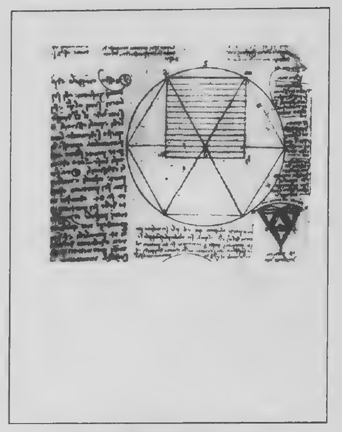Transparency 14-R-2: Da Vinci’s attempt to square the circle

is the race called the Indianapolis 500? (Because it is 500 miles long.) How many times do the cars go around the track? (200.) How long does it take a car traveling 200 miles per hour to go once around the track? (45 seconds.)

What is the area of the region enclosed by the track? (Approximately 0.41 square mile.) The discussion of these calculations leads easily into a consideration of the topics of the new lesson: arc lengths, and sectors and their areas.

Review of Chapter 14

Transparencies

• 14-R-1 King Arthur’s Round Table
• 14-R-2 Da Vinci’s attempt to square the circle
• 14-R-3 Squaring a crescent

First day

Introduction

The drawing on Transparency 14-R-1 is of King Arthur’s Round Table and is from the “Prince Valiant” comic strip. You might ask your students to imagine that King Arthur and one hundred of his knights are seated at a round table and each person takes up two feet of the table’s circumference. How far is each man from the people seated farthest from him? (The men are at the vertices of a regular polygon having 101 sides. The problem is to find the length of one of its longest diagonals. The longest diagonals are slightly shorter than a diameter of the circle, but close enough to it that its length can be

used for the calculation. d = c/π = 2,002/π ≈ 64. The distance is about 64 feet.)

Second day

Introduction

One of the most famous problems in geometry is that of squaring the circle. To “square a circle” means to use only a straightedge and compass to construct a square that is equal in area to a given circle. Leonardo da Vinci devoted many hours to this problem. Part of a page of one of his notebooks in which he wrote about it is shown on Transparency 14-R-2. It was not until 1882 that it was proved that, like trisecting an angle, the problem of squaring the circle will never be solved.

Show Transparency 14-R-3. In the fifth century B.C., a Greek mathematician named Hippocrates discovered, in trying to square the circle, how to square the crescent-shaped region in this figure. Describe the figure as your students construct it. △ABC is an isosceles right triangle and D is the midpoint of its hypotenuse. The center of CEB is point A and the center of CFB is point D. Let DB = x. The area of the “crescent” can be expressed in terms of x by noticing that it is the difference of the areas of the circular segments CBFC and CBEC. The area of the segment CBEC, in turn, is the difference of the areas of the sector △BEC and △ABC. Using these clues, see if you can find an expression for the area of the “crescent” in terms of x.

Drawing DA forms isosceles right △ABD, and so AB = x√2.

αCEBFC = αCBFC − αCBEC = αCBFC − (αABEC − αΔABC) = ½πx² − [¼π(x√2)² − ½(x√2)²]

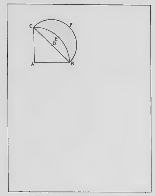Transparency 14-R-3: Squaring a crescent

Using this result, can you think of a simple way to “square the crescent” by adding a square to the figure? (Because the area of the square is x², its side is x. DA and DB might be used as two sides of the square.)

According to the Greek historian Proclus, Hippocrates, who first figured all of this out, wrote an “Elements of Geometry” more than a century before Euclid wrote his Elements, but Hippocrates’ book, like most mathematical writing of that time, has been lost.

Transparency 15-1-1: File-card puzzle

Transparency 15-1-2: Church porch

Figure on page 394 — A rectangle divided into a square and a smaller similar rectangle (golden-rectangle construction)

Chapter 15: Geometric Solids

Lesson 1: Lines and Planes in Space

Lesson Outline

Terms: Skew lines, parallel planes (or line and plane), perpendicular line and plane, perpendicular planes, oblique planes (or line and plane).

Transparencies

• 15-1-1 File-card puzzle
• 15-1-2 Church porch

Introduction

The figure on Transparency 15-1-1 once appeared in the “Mathematical Games” column of Scientific American and was said to have been in an entrance examination for the School of Architecture of the University of Leningrad. The problem was to make amodel of the figure by taking an ordinary file card, cutting it with scissors, and folding it. In his column, Martin Gardner referred to it as a marvelous test of one’s ability to think in three-dimensional space.*

To introduce the lesson, give each of your students an unlined file card and a pair of scissors to try to create a three-dimensional model of the figure. After some of your students have succeeded at

this, you might draw the following figure on the transparency as a clue on what to do.

The figure on Transparency 15-1-2 is another challenge to our ability to think in three-dimensional space. It is a design for a church porch.* An appropriate sign to put over the entrance would be “Abandon hope, ye who would enter here!” Why? (Bending a sheet of paper in the shape of the walls and ceiling over the door should reveal what is wrong.)

‘This figure is from Perspective in Perspective by Lawrence Wright (Routledge and Kegan Paul, 1983).

*“Mathematical Games,” by Martin Gardner, Scientific American, November 1978.

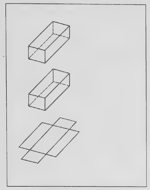Transparency 15-2-1: Rectangular solid

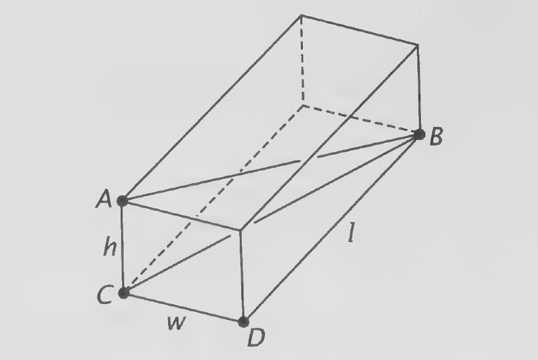Figure on page 395 — A rectangular box with its length, width, height, and space diagonal labelled

Lesson 2: Rectangular Solids

Lesson Outline

Terms: Polyhedron, rectangular solid, diagonal and dimensions of rectangular solid, cube.

Theorem 79. The length of a diagonal of a rectangular solid with dimensions l, w, and h is √(l² + w² + h²).

Corollary. The length of a diagonal of a cube with edges of length e is e√3.

Transparencies

• 15-2-1 Rectangular solid

Introduction

Before class, stretch a cord or a piece of brightly colored yarn diagonally across the room from one of the corners of the ceiling to the opposite corner of the floor. Begin class by handing out small pieces of paper. Remark that the subject of today’s lesson is rectangular solids and that the classroom is a good example of a rectangular solid. Explain that the cord represents a diagonal of the room, and ask your students to guess its length in feet, writing their names and their guesses on the pieces of paper you have given them. Collect the guesses and set them aside.

Had out duplicated copies of Transparency 15-2-1 and have your students draw diagonal AB in the first figure, as shown at the right. Also label points C and D, and the dimensions of the room h, w, and |.

Explain that the length of AB is determined by the dimensions of the room. To see how this is done, draw CB to form a triangle with AB as one of its

sides. After your students have noticed that △ABC and △BCD are right triangles, guide them in applying the Pythagorean Theorem to the figure to derive the formula for the length of a diagonal of a rectangular solid. (This can be done at the right of the first figure.)

Then, give the dimensions of your classroom in feet and have your students write them on the second figure. Ask them to use the formula that they have just derived to calculate the length of the diagonal. (My classroom is 27 feet wide, 31 feet long, and 14 feet high, and so the length of the diagonal is 1,886 ≅ 43.4 feet.) While your students are doing this, sort out their guesses. After the calculation has been discussed, announce the name(s) of the students(s) who came closest. It might also be interesting to tell the smallest and largest guesses without telling the names of the students who guessed them. (The extreme guesses usually turn

Transparency 15-3-1: Photograph of crystals

Transparency 15-3-2: Cover of Crystal Geometry

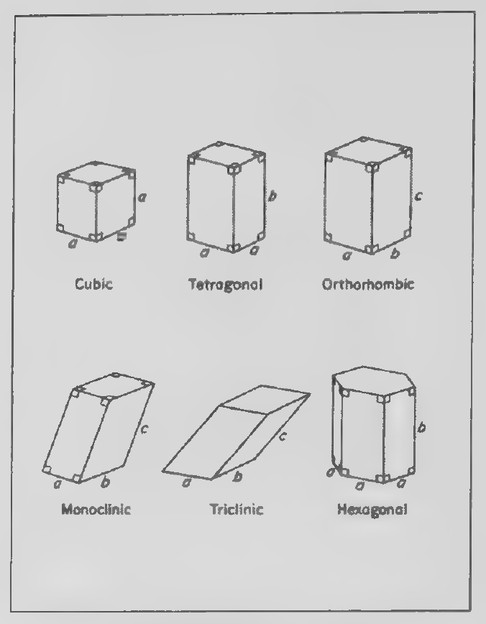Transparency 15-3-3: A page from Crystal Geometry

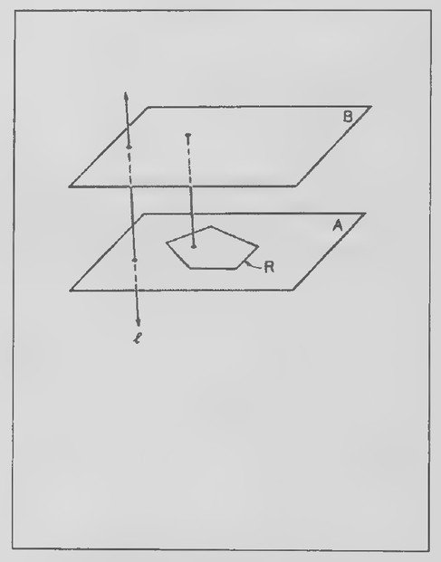Transparency 15-3-4: A prism

out to be quite outlandish.)

The third figure of the transparency might be used to derive the formula for the surface area of a rectangular solid. The figure can be thought of as the floor and walls of the room, collapsed outward. Have your students add a sixth rectangle at the right to represent the ceiling. Then label the dimensions of the rectangles in terms of I, w and h and use the figure to find the surface area formula. For practice, your students might calculator the total surface area of your classroom in square feet.

To close the lesson, you might guide your students in writing formulas for the length of a diagonal of a cube and its surface area. It is helpful to compare the formulas for the lengths of the diagonals of a square and a cube, emphasizing that both formulas contain square roots and asking your students how they might remember that the square formula has a 2 in it and the cube formula has a 3.

Lesson 3: Prisms

Lesson Outline

Terms: Prism, bases, lateral faces and edges, right prism, oblique prism, net, lateral area, total area of prism.

Transparencies

• 15-3-1 Photograph of crystals
• 15-3-2 Cover of Crystal Geometry
• 15-3-3 A page from Crystal Geometry
• 15-3-4 A prism

Introduction

The pictures on Transparency 15-3-1 are photo-

graphs of crystals. The two solids at the top are sodium chlorate crystals and the solid at the bottom is a crystal of chrome alum. Many minerals have crystals in the shape of polyhedra. The figure on the dust jack of Introduction to Crystal Geometry (Transparency 15-3-2) suggests why.* Crystals are three-dimensional arrangements of atoms in which the atoms line up in rows that result in straight edges and flat surfaces.

Crystals can be imagined to consist of little building blocks. Each building block corresponds to an arrangement of atoms or molecules that is regularly repeated throughout the crystal.

“Introduction to Crystal Geometry by Martin J. Buerger (McGraw-Hill, 1971).

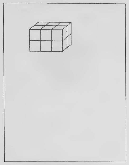Transparency 15-4-1: Cubes in box problem

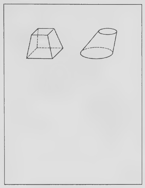Transparency 15-4-2: Cavalieri’s Principle

Every crystal belongs to one of the six crystal systems illustrated on Transparency 15-3-3. Each system uses a different type of building block and it is the shapes of the building blocks that are shown. Notice that the first three shapes are rectangular solids. All six shapes are prisms.

Following this introduction, you can use Transparency 15-3-4 and its overlay to make the general definition of a prism clear. The rest of the lesson can be presented as in the text.

Lesson 4: The Volume of a Prism

Lesson Outline

Terms: Altitude of a prism, volume, cross section

Postulate 13. Cavalieri’s Principle. Consider two geometric solids and a plane. If every plane parallel to this plane that intersects one of the solids also intersects the other so that the resulting cross sections have equal areas, then the two solids have equal volumes.

Postulate 14. The volume of any prism is the product of the area of its base and its altitude: V=Bh

Corollary 1. The volume of a rectangular solid is the product of its length, width, and height: V =lwh.

Corollary 2. The volume of a cube is the cube of its edge: Vice.

Transparencies

• 15-4-1 Cubes in box problem
• 15-4-2 Cavalieri’s Principle

Introduction

Transparency 15-4-1 can be used to introduce the new lesson. The figure on it appeared in a mathematics question in a test of the National Assessment of Educational Progress. The question was: How many cubes does the box contain?

After discussing the answer, your students might be interested to know that of the 9-year-olds asked this question, only 6% answered it correctly. Of the people 13 years old, 21% gave the correct answer, and of those 17 years old, only 43%! The most commonly given wrong answer was “16.”

After observing that the volume of a rectangular solid that has been divided into unit cubes can be found by counting them, explain that not every solid can be divided into cubes. To find the volume of a general prism, we need to make some assumptions. First, introduce the V = lwh and V = Bh formulas for rectangular solids as in the text. Then, use a deck of playing cards or a ream of paper to suggest how the volume of an oblique rectangular prism might be found from a right rectangular prism. Transparency 15-4-2 and its overlay can be used to introduce Cavalieri’s Principle and the rest of the lesson presented as in the text.

Transparency 15-5-1: Photograph of the Great Pyramid

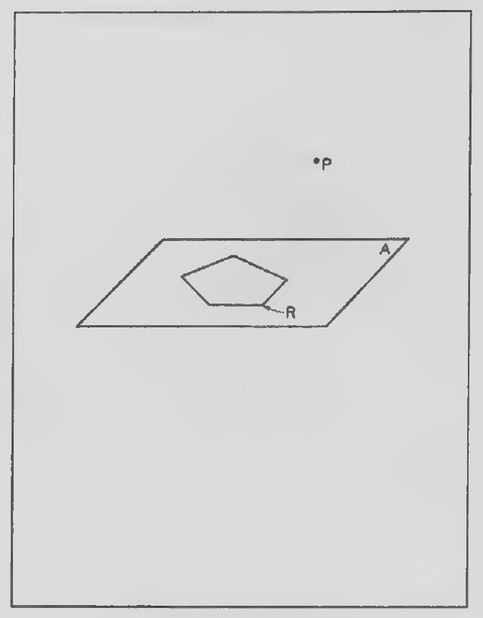Transparency 15-5-2: A pyramid

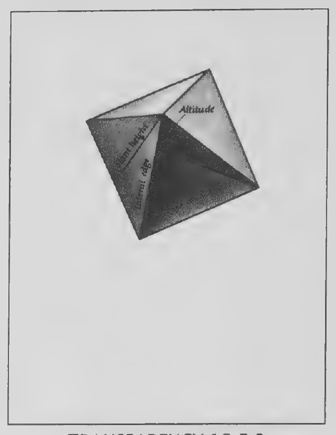Transparency 15-5-3: Great Pyramid

Lesson 5: Pyramids

Lesson Outline

Terms: Pyramid, base, lateral faces and edges, apex, altitude of pyramid Theorem 80. The volume of any pyramid is onethird of the product of the area of its base and its altitude: Ve = Bh 3

Transparencies

• 15-5-1 Photograph of the Great Pyramid
• 15-5-2 A pyramid 15-5-3. A square pyramid

Worksheet: Three pyramids that fold into

a cube 15-5-4 Three pyramids that fold into a cube

Introduction

The word “pyramid” usually brings to mind the pyramids of Egypt. The Great Pyramid, shown in the photograph on Transparency 15-5-1, is certainly the most famous example. Its shape suggests that a pyramid has a square base and triangular faces that meet at a point. For pyramids in general, however, this is only partly true. Use Transparency 15-5-2 and its overlay to present the geometric definition of a pyramid.

Explain that the Great Pyramid of Egypt is an example of a square pyramid, hand out duplicated copies of Transparency 15-5-3, and introduce the terms pictured onit. Then have your students write on the figure the length of an edge of the base of the Great Pyramid, 760 ft, and its altitude, 484 ft. Guide

them in using the appropriate right triangles to find the altitude of one of the faces (615 ft) and the length of a lateral edge (723 ft).

Hand out scissors and copies of the pattern on Worksheet for Lesson 15-5. (If possible, print the worksheet on cover stock; note that there are two patterns on each sheet.) Explain to your students that they are going to do an experiment that will enable them to guess a formula for the volume of a pyramid. Tell them to cut out the pattern, fold it along all the lines, and see what they notice. After they have had time to do this, ask someone to describe what they have noticed.

The pattern can be folded into three square pyramids (unlike the Great Pyramid, their lateral edges are not equal), which can, in turn, be folded toward each other to form a cube. Transparency 15-5-4 illustrates how this can be done. Note that the three pyramids seem to be identical, and so they have equal volumes. Because they can be folded together to form a cube, its volume is three times that of each pyramid. Hence, the volume of one of the pyramids is one-third that of the cube. Because the cube and pyramids have equal bases and altitudes, the volume of one of the pyramids is evidently one-third the product of the area of its base and its altitude. Explain that this conclusion is true for all pyramids and that we will consider it a theorem even though we have not proved it.

To conclude the new lesson, show Transparency 15-5-3 again and help your students, as needed, to find the lateral area and volume of the Great Pyramid. (They are approximately 935,000 square feet and 93,200,000 cubic feet, respectively.)

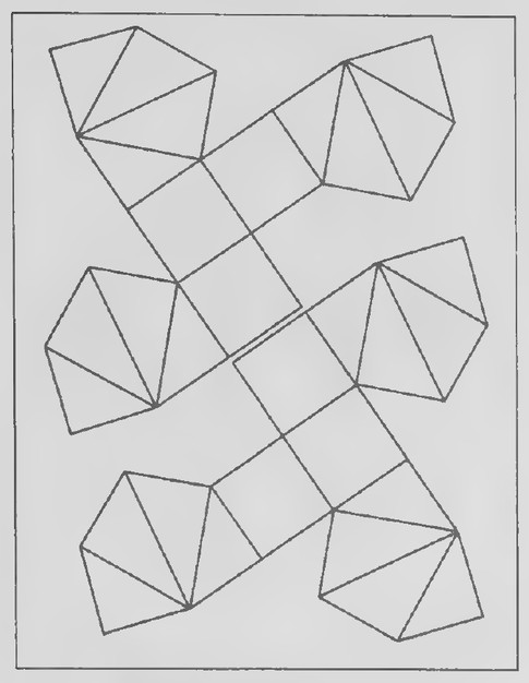WORKSHEET FOR 15-5

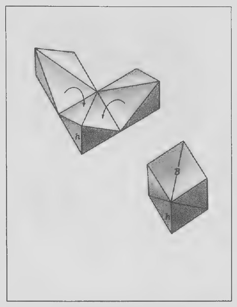Transparency 15-5-4: Three pyramids that fold into a cube

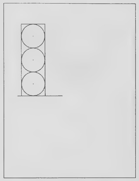Transparency 15-6-1: Can of tennis balls

Lesson 6: Cylinders and Cones

Lesson Outline

Terms: Cone, lateral surface, circular region, base, apex, altitude, axis, right and oblique cones, cylinder, bases, lateral surface, altitude, axis, right and oblique cylinders.

Theorem 81. The volume of a cylinder is the product of the area of its base and its altitude: V =Bh=rrh.

Theorem 82. The volume of a cone is one-third the product of the area of its base and its altitude:

V= oR, = Lee 3 3

Transparencies

15-6-1_ A can of tennis balls

Introduction

Cut a strip of paper so that it will exactly fit when it is wrapped around a can of tennis balls. Tape the ends of the strip together so that it is held securely in place around the can. Start class by holding up the can and describing what you have done. Tell your students that you are going to cut the strip where you have taped it and stretch it beside the can, holding one end at the bottom. How high would the other end reach?

Hand out duplicated copies of Transparency 15-6-1 which contains a figure representing the can with the three balls inside it. Ask your students to draw a line segment upward from the bottom line to represent how far they think the strip of paper would stretch, While they are doing this, you might

hold the can toward them so that they can see the size of its circular cross section.

Almost all of my students guess that the length of the strip is less than the height of the can. Without telling your students the answer, have them draw asegment through the centers of the balls from the bottom to the top of the can. Label the radii of the circles representing the balls r. What is the height of the can in terms of r² (6r.) What is the length of the strip of paper? (It is the circumference of the base of the can: 2nr, or approximately 6.28r.) So the length of the strip is more than the height of the can!

Following this introduction, the lesson on cylinders and cones can be presented as in the text.

Transparency 15-7-1: Cork ball

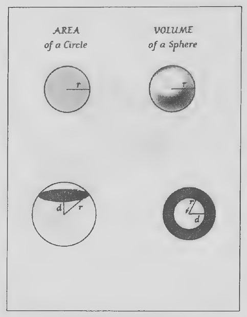Transparency 15-7-2: Circle and sphere

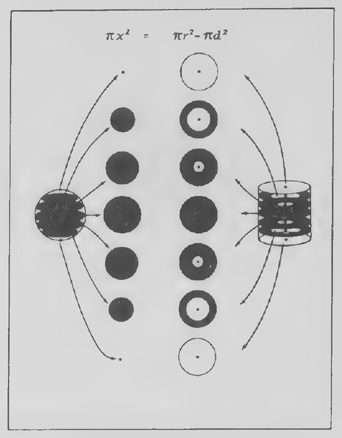Transparency 15-7-3

Lesson 7: Spheres

Lesson Outline

Terms: Sphere, center, radius, diameter

Theorem 83. The volume of a sphere is on times the cube of its radius:

=3™- ee

Theorem 84. The surface area of a sphere is 4r times the square of its radius: A= ary

Transparencies

• 15-7-1 Cork ball
• 15-7-2 Circle and sphere 15-7-3. Cross sections of a sphere
• 15-7-4 Asphere and hollowed-out cylinder
• 15-7-5 Recreational sites on Mercury
• 15-7-6 The surface area of a sphere

First day

Introduction

Here is a good puzzle.*

You know how very light cork is. When you have a cork stopper in hand—just now taken out of a bottle—it weighs practically nothing. If thrown into a bowl of water it floats hardly submerged. The stuff is very, very light. So—quick now—we have a ball of cork—a sphere of cork−5 feet in diameter. Ques-

tion: What does it weigh? Could you lift it? No calculations! Just give us a quick guess.

(Show Transparency 15-7-1 and ask your students to write their guesses before continuing.) In order to figure out what a ball of cork 5 feet in diameter would actually weigh, we need to know two things: the density of cork—that is, how much a given volume of it weighs—and, how to find the volume of a sphere.

One cubic inch of cork weighs about 0.14 ounce. To find out how many cubic inches of cork there would be ina ball 5 feet in diameter, we need a formula for the volume of a sphere.

(Show the top half of Transparency 15-7-2.) We know that the area of a circle is a little more than three times the square of its radius: more precisely, mr’. Would you expect the volume of a sphere to also be measured in terms of the square of its radius? (No. Since volume is measured in cubic units, it should be some number times the cube of the radius: that is,?r°.) To find this number, we can use Cavalieri’s Principle.

In deriving the formula for the volume of a sphere, it is helpful to have some models. I use two 4.5-in diameter Styrofoam spheres (available in art and crafts stores), one of which I have sliced into two pieces as in the figure on page 663 of the text. I also use a model of the hollowed-out cylinder (also shown on page 663) whose dimensions match those of the spheres. This model can be made from tag board and tape.

I have my students make a drawing showing a side view of the sphereas shown in the next column.

*From Millergrams I, by Julius Sumner Miller (Doubleday, 1970).

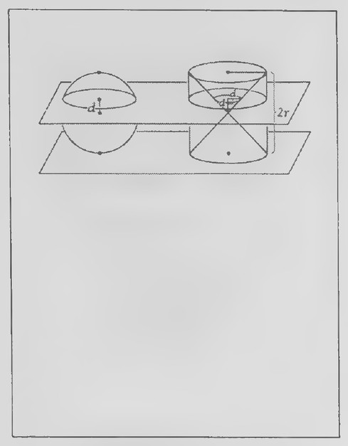Transparency 15-7-4: Asphere and hollowed-out cylinder

Transparency 15-7-5: Recreational sites on Mercury

Transparency 15-7-6: The surface area of a sphere

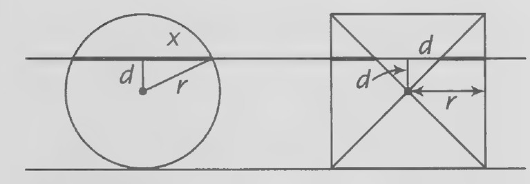Figure on page 401 — A circle of radius r and diameter d inside a square, illustrating the area relationship

T(r² - d²) Trré - trd2

We treat the discovery of the hollowed-out cylinder as a detective story, illustrating it first with a square and then adding the details step by step. The figures on Transparencies 15-7-3 and 15-7-4 should also be helpful in enabling your students to understand the volume derivation.

After the volume formula has been derived, show Transparency 15-7-2 again and note that we have found the number we were looking for: it is

of Then return to Transparency 15-7-1 and find

the volume and weight of the cork ball.

Since the diameter of the ball is 5 feet, its radius is 2.5 feet or 30 inches:

4

Viait = 3730)? = 36,000n

= 113,000 cubic inches.

Since one cubic inch of cork weighs about 0.14 ounce, the ball would weigh 113,000(0.14) = 15,820 ounces, or almost half a ton!

Since this lesson covers a lot of material, I suggest not assigning any problems for homework until the next day.

Second day

Introduction

Earlier in the course, we calculated the cost of an acre of land in the Yukon Territory that was being sold for 25¢ per square inch. Omni magazine once reported that the Astronomical Society of the Pacific was selling recreational sites on the planet Mercury (Transparency 15-7-5). The sites are advertised as “pollution-free and also atmosphere-free,” but buyers are also warned that the temperatures are somewhat balmy (actually, hot enough to melt lead). At the rate of $25 for 14,000 acres, how much would it cost to buy the entire planet?

To be able to answer this question, we need to know how to find the surface area of a sphere. Use Transparency 15-7-6 to derive the formula for the surface area of a sphere as in the text and then return to the problem about Mercury as a class exercise.

The diameter of Mercury is 3,100 miles and 1 square mile is equal to 640 acres. The surface area of the planet is 4n(1,550)? = 30,000,000 square miles. At $25 for 14,000 acres, the entire planet would cost approximately 35 million dollars.

The Society that made the land offer is a nonprofit organization dedicated to increasing public understanding of astronomy and admits that it does not actually own any land on Mercury.

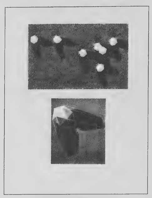Transparency 15-9-1: Icosahedral virus

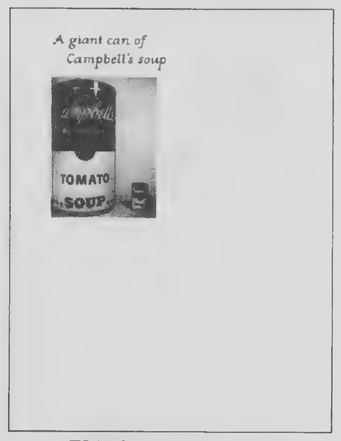Transparency 15-8-1: A giant can of Campbell’s soup

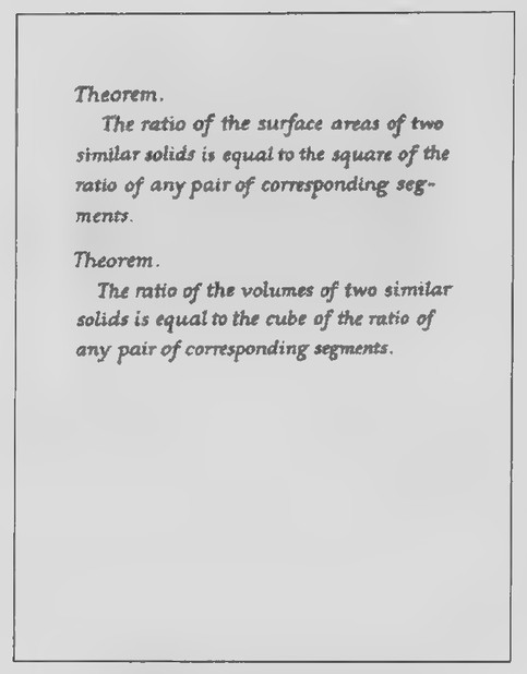Transparency 15-8-2: Similar solids theorems

Figure on page 402 — A cylinder and the inscribed rectangular prism used to compare their volumes, with dimensions labelled

Lesson 8: Similar Solids

Lesson Outline

Terms: Similar solids. Theorem 85. If the ratio of a pair of corresponding dimensions of two similar solids is r, then the ratio of their surface areas is r². Theorem 86. If the ratio of a pair of corresponding dimensions of two similar solids is r, then the ratio of their volumes is 7°.

Transparencies

• 15-8-1 A giant can of Campbell’s soup
• 15-8-2 Similar solids theorems

Introduction

An amusing way to introduce this lesson is with a large wastebasket that has been painted to look like a can of soup or soda. The photograph on Transparency 15-8-1 shows a large “Campbell’s soup can” that I bought at a novelty store. An actual can of soup stands beside it.

Although this giant can is a wastebasket, it looks very much like a can of Campbell’s soup. It is about five times as tell as an actual can and has about five times its diameter. As a result, the two cans, giant and genuine, have the same shape.

Have your students draw pictures of two cylinders to represent the cans and label their dimensions as indicated in the figure at the right. If two geometric solids are similar, every pair of distances between pairs of corresponding points in the two

ay ete eae solids is proportional. If the cans are similar, — = — =r.

a (Explain that r represents the ratio of the correspond-

ing dimensions and that in the case of the cans, r=5.) Note that c= ra and d = rb.

How do the lateral areas of the two cans compare? For the small can, A = 2nab, and for the giant can, A = 2ncd = 2n(ra)(rb) = r2(2rab). The ratio of the lateral areas is r². Because r = 5, the lateral area of the giant can is 5¢ = 25 times that of the small can. The “label” on the giant can, then, is 25 times as large as the label on the small can.

How do the volumes of the two cans compare? For the small can, V = 71a@*b, and for the giant can, V = nc2d = n(ra)2(rb) = r3(na2b). The ratio of the volumes is 73. The volume of the giant can is 5° = 125 times that of the small can.

3

The actual can of soup weighs 10 4° and costs

99¢ (at the time of writing). If the giant can were

Transparency 15-R-1: Five intersecting cubes

Transparency 15-R-2: THE STEREOCHEMICAL THEORY OF ODOR

Transparency 15-R-3: Table: Primary odors

filled with soup, how much do you think it would weigh and cost? (Having 125 times the volume of the small can, it is reasonable to think that it would weigh 125 times as much, or about 84 lb. If it also costs 125 times as much, it would cost $123.75.)

Suppose that an even larger can, still similar in shape to the small one, was ten times as tall. How many times bigger do you think its label, weight, and cost would be? (Because r = 10, r² = 100 and r = 1,000. The large can would have a label 100 times as large and would weigh and cost 1,000 times as much.)

Show Transparency 15-8-2 and explain that these theorems hold true, not just for similar cylinders, but for any pair of similar solids. Point out that it is easy to remember that the area ratio is found by squaring and that the volume ratio is found by cubing because area and volume are measured in square and cubic units, respectively.

Lesson 9: The Regular Polyhedra

Lesson Outline

Terms: Regular polyhedron, tetrahedron, octahedron, icosahedron, dodecahedron.

Transparencies

• 15-9-1 Icosahedral virus

Introduction

The photograph at the top of Transparency 15-9-1 was taken through an electron microscope and shows particles of a virus enlarged about 58,000 times. Note the double shadows of the particles and the constancy of their shape. A geometric solid that

casts shadows exactly like these particles is pictured at the bottom of the transparency. It is called an icosahedron and, because its shadows match those of the virus, biologists think that the particles of the virus are in the shape of tiny icosahedra. Models like those shown on page 678 of the text would be helpful in introducing the other regular polyhedra.

Review of Chapter 15

Transparencies

• 15-R-1 Five intersecting cubes 15-R-2. “The Stereochemical Theory of Odor”
• 15-R-3 Table: Primary odors
• 15-R-4 Olfactory receptor sites
• 15-R-5 Analmond odor

First day

Introduction

The polyhedron pictured on Transparency 15-R-1 is very complex and yet very simple. Its edges form equilateral triangles, squares, regular pentagons, and five-pointed stars, and it contains 360 faces in all. The 360 faces do not lie in 360 different planes, however. They are contained in only 30 planes and this is what makes the polyhedron simple. Perhaps some of your students will be able to recognize that there are large cubes hidden in the polyhedron. The overlay can be put on the transparency to reveal one of these cubes.

I made the model in the photograph from cardboard and tape, with sticks of balsa wood inside to make it rigid. Information on the patterns needed is given on page 136 of Mathematical Models, Revised Edition, by H. Martyn Cundy and A. P. Rollett (Ox-

Transparency 15-R-4: Olfactory receptor sites

Transparency 15-R-5: Analmond odor

ford University Press, 1961), but its construction requires a lot of time and patience.

Second day

Introduction

Take one or two bottles of almond extract and either remove or tape over the labels so that the names are covered. Hand the bottle(s) out at the beginning of class and ask your students to try to identify the odor.

A Roman poet and philosopher named Lucretius speculated two thousand years ago that the sense of smell is based on geometry. He thought that every substance that has an odor gives off tiny particles of a specific shape. When these particles enter a person’s nose, they fit into certain pores that match their shape. The pores into which the particles fit enable the person to identify the substance from which they came.

Modern scientists now think that Lucretius’s theory is correct. Show Transparency 15-R-2, on which the first page of an article on odor that appeared in Scientific American is reproduced.* Note the sentence under the title stating that “there is evidence that the sense of smell is based on the geometry of molecules.” There seem to be seven basic odors, as listed in the table enlarged from the article on Transparency 15-R-3. Each of the first five is associated with molecules of a particular geometric shape. Show Transparency 15-R-4. These figures

show perspective, top, and side views of the receptor sites for these five odors. The camphoraceous site is hemispherical in shape. The site corresponding to the odor of musk is shaped like a cylinder. Those for floral and pepperminty odors are more complex in shape, whereas the ethereal site is long and rod-shaped. Add the overlay to the transparency. These diagrams represent molecules that fit each of the five sites.

The two basic odors not shown here, pungent and putrid, are determined not by the shape of the molecule but rather by its charge. Pungent odors, such as that of vinegar, are caused by positively charged molecules, whereas putrid odors are caused by molecules that are negatively charged.

By this time, everyone should have had a chance to smell the almond extract. After someone has identified it, show Transparency 15-R-5. It appears that all odors can be explained in terms of the seven basic ones. For example, the odor of almonds is a combination of camphoraceous, floral, and pepperminty odors. Molecules that possess this odor can fit any one of the three sites (actually, two of them in the floral site). Aremarkable consequence of this theory is that, by putting their knowledge of three-dimensional geometry to use, chemists have been successful in synthesizing substances having various odors simply by producing molecules of the right shape.

*This lesson and its illustrations are adapted from “The Stereochemical Theory of Odor” by John E. Amoore, James W. Johnston, Jr., and Martin Rubin, Scientific American, February 1964, pages 42-49.

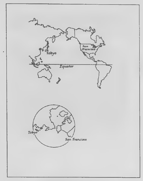WORKSHEET 16-1

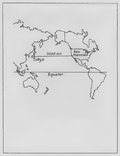Transparency 16-1-1: From San Francisco to Tokyo

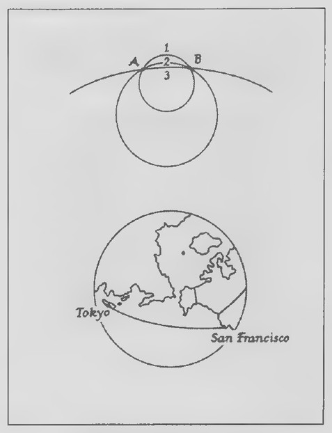Transparency 16-1-2: The great circle route

Chapter 16: Non-Euclidean Geometries

Before beginning to teach this chapter, it may be helpful to read the following articles:

“Euclid’s Parallel Postulate and Its Modern Offspring” by Martin Gardner, Scientific American, October 1981, pages 23-33.

Mathematics in Western Culture by Morris Kline (Oxford University Press, 1953), Chapter 26, “New Geometries, New Worlds.”

Einstein’s Legacy by Julian Schwinger (Scientific American Books, 1986), Chapter 5, “Geometry and Physics.”

Another valuable reference is the book Euclidean and Non-Euclidean Geometries, Second Edition, by Marvin Jay Greenberg (W. H. Freeman and Company, 1980).

Lesson 1: Geometry on a Sphere

Lesson Outline

Terms: Great circle, antipodal points.

Transparencies

• 16-1-1 From San Francisco to Tokyo
• 16-1-2 The great circle route

Introduction

Hand out duplicated copies of Worksheet for Lesson 16-1. Here are two maps showing the cities of Tokyo and San Francisco. Suppose that a ship sails

from one city to the other. Use your pencil to mark on the first map the path of the ship.

After your students have done this, show Transparency 16-1-1. Gerardus Mercator, the Flemish cartographer who devised the method of mapping the earth used here, wrote:

If you wish to sail from one point to another, here is a chart, and a straight line on it, and if you follow this line carefully you will certainly arrive at your destination. But the length of the line may not be correct. You may get there sooner or may not get there as soon as you expected but you will certainly get there.*

Mercator was referring to a problem that many people are not aware of when they look at a map such as his. It would seem that any other path between Tokyo and San Francisco would be longer than the one we have drawn, yet here is a path (add the overlay to Transparency 16-1) that is significantly shorter. Can you explain how this can be?

Because these paths are on the surface of a sphere, neither one is straight. Both, in fact, are arcs of circles. Show Transparency 16-1-2. In the top figure, two points, A and B, are joined by three arcs numbered 1, 2, and 3. Which arc is shortest? (Arc 3.) How does the circle of which it is a part compare

*From Mapping by David Greenhood (University of Chicago Press, 1964), page 128.

Transparency 16-2-1: What if the world were cubical?

Transparency 16-2-2: What if the world were conical?

Transparency 16-2-3: What if the world were toroidal?

with the other circles? (It is the largest.) If you could not draw a straight line through points A and B, but could only draw a circle, what would you do to make the arc from A to B as short as possible? (Make the circle as large as possible.)

Look at the bottom figure of the transparency. Because Tokyo and San Francisco are on the surface of a sphere, we cannot draw astraight line along it from one point to the other. We will have to settle for a circle instead. How should we choose it to make the arc from A to Bas short as possible? (Choose the largest possible circle through A and B that lies on the surface of the sphere; namely, the circle whose radius is the same as that of the sphere.) Add the overlay to Transparency 16-1-2 and explain the idea of a great circle. Now have your students mark the center of the earth on the second figure on their worksheets and sketch the great circle that goes through Tokyo and San Francisco.

The rest of the lesson can be developed as in the text.

Lesson 2: The Saccheri Quadrilateral

Lesson Outline

Terms: Birectangular quadrilateral: base, legs, summit, base angles, summit angles; Saccheri quadrilateral.

Theorem 87. The summit angles of a Saccheri quadrilateral are equal.

Theorem 88. The line segment connecting the midpoints of the base and summit of a Saccheri quadrilateral is perpendicular to both

of them. Theorem 89. If the legs of a birectangular quadrilat-

eral are unequal, the summit angles opposite

them are unequal in the same order. Theorem 90. If the summit angles of a

birectangular quadrilateral are unequal, the

legs opposite them are unequal in the same

order.

Transparencies

• 16-2-1 What if the world were cubical?
• 16-2-2 What if the world were conical?
• 16-2-3 What if the world were toroidal?
• 16-2-4 What if the world were cataclysmal?
• 16-2-5 Euclid’s fifth postulate
• 16-2-6 Geometry books
• 16-2-7 A deductive system

Introduction

Joseph N. Portney has designed a very attractive set of 9-in x 12-in posters on the theme “What if the world were…?” There are twelve posters in the set, showing photographs of models of an earth that is flat, cubical, dodecahedral, pyramidal, cylindrical, conical, toroidal, hyperboloidal, hyperbolic paraboloidal, oblate spheroidal, “Wegeneroidal,” and “cataclysmal.” The set can be seen on http:/ / www.nrich.maths.org.uk/mathsf /journalf/dec99/ art1/. The figures on Transparencies 16-2-1, 16-2-2, 16-2-3, and 16-2-4 are taken from these posters.

You know that the shortest path between two points in a plane is the line segment joining them. What is the shortest path between two points on a sphere? (An arc of a great circle.) What do you think the shortest path between two points on the sur-

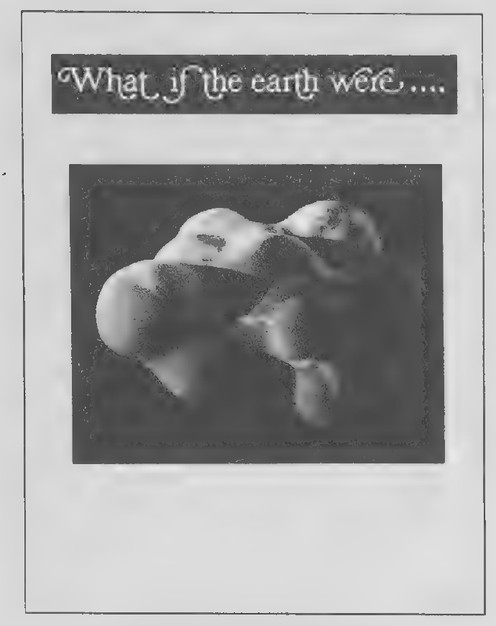Transparency 16-2-4: What if the world were cataclysmal?

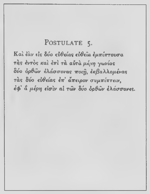Transparency 16-2-5: Euclid’s fifth postulate

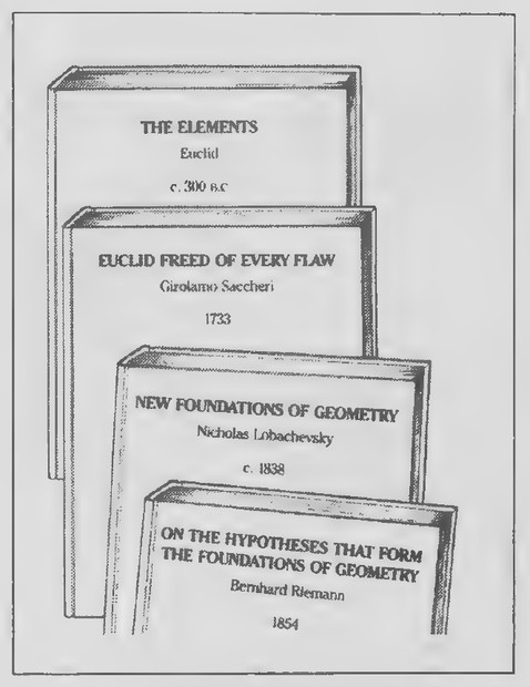Transparency 16-2-6: Geometry books

face of a cube would be? (A set of one or more line segments.) The shortest paths on the cone and toroid are more complicated and on the “cataclysmal” surface, extremely complex.

To introduce the new lesson, you might show Transparency 16-2-5. Perhaps the most controversial statement to be made in all of the history of mathematics is Euclid’s fifth postulate. Shown here in the original Greek, the postulate states, in effect, that through a point not on a line, there is exactly one line parallel to the line.*

What made the postulate controversial is not that people did not believe it, but rather that others thought Euclid should have proved it as a theorem. Show Transparency 16-2-6. One person who thought this was an Italian priest named Saccheri and who went so far as to write a book titled Euclid Freed Of Every Flaw in which he tried to prove the Parallel Postulate. In this lesson, we will see how Saccheri set out to do this.* The rest of the lesson can now be presented as in the text.

Be sure to emphasize that because Saccheri was trying to prove the Parallel Postulate, he could not

use any theorems whose proofs depend on it. The diagram on Transparency 16-2-7 should help clarify the situation. The boxes represent postulates and the circle identify by number some of the theorems that depend on these postulates. The arrows show only a few of the relations between the statements in the system. In essence, we cannot use any theorems in the bottom group as we prove the theorems in this lesson. You may want to show the transparency from time to time as questions arise. For example, some students will concluce that because the summit angles of a Saccheri quadrilateral are equal, it must be a rectangle. This follows from Theorem 32 (the sum of the measures of the angles of a quadrilateral is 360°). But the proof of Theorem 32 uses Theorem 28 (the sum of the measures of the angles of a triangle is 180°). Theorem 28, in turn, follows from Theorem 25, which follows from the Parallel Postulate. Therefore, if the purpose of the Saccheri quadrilateral is to prove the Parallel Postulate, we cannot assume that it is a rectangle.

The proofs of the four theorems are outlined in the exercises. The proofs of the theorems not assigned should be demonstrated in the lesson.

*This is known as “Playfair’s postulate” and is, of course, the version of the Parallel Postulate that we have used throughout the course. Euclid’s version is: “That, if a straight line falling on two straight lines makes the interior angles on the same side less than two right angles, the two straight lines, if produced indefinitely, meet on that side on which are the angles less than the two right angles.” I would not bring this up in the lesson. tThe article “Saccheri, Forerunner of Non-Euclidean Geometry” by Sister Mary of Mercy Fitzpatrick in The Mathematics Teacher (May 1964), pages 323-332, is a valuable reference.

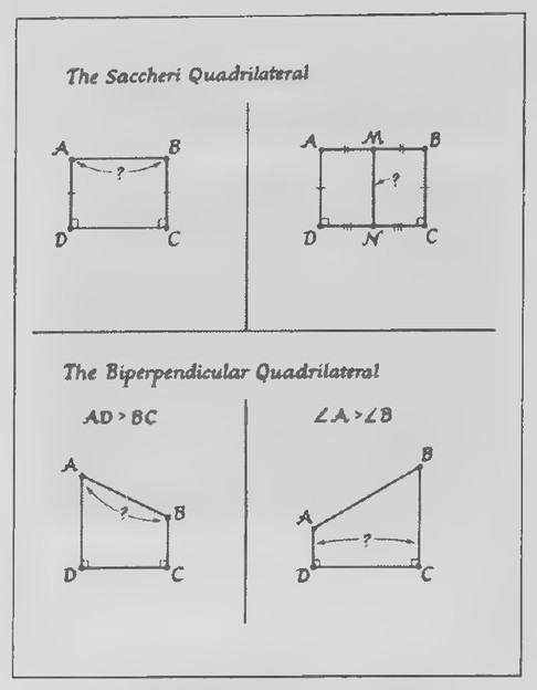Transparency 16-3-2: Review of Theorems 87 through 90

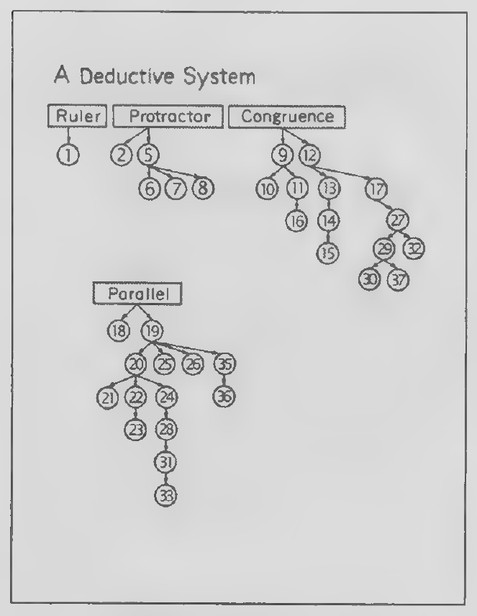Transparency 16-2-7: A deductive system

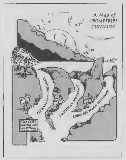Transparency 16-3-1: A Map of

Lesson 3: The Geometries of Lobachevsky and Riemann

Lesson Outline

Terms: The Lobachevskian Postulate. The summit angles of a Saccheri quadrilateral are acute.

Lobachevskian Theorem 1. The summit of a Saccheri

quadrilateral is longer than its base.

Lobachevskian Theorem 2. A midsegment of a

triangle is less than half as long as the third side.

Transparencies

16-3-1_ Map: Geometries country 16-3-2 Review of Theorems 87 through 90 16-3-3 Theorem 87 (Lesson 2: Set I, Exs. 7-13) 16-3-4 Theorem 88 (Lesson 2: Set II, Exs. 31-35) 16-3-5 Theorem 89 (Lesson 2: Set I, Exs. 14-21) 16-3-6 Theorem 90 (Lesson 2: Set I, Exs. 22-28) 16-3-7 Table: Comparing three geometries

Introduction

To open this lesson, show Transparency 16-3-1. This map compares our study of geometry to traveling through the country. Earlier in the course, we came to the junction pictured at the bottom of the map. When we assumed the Parallel Postulate—that is, that through a point not on a line, there is exactly one line parallel to the line—we chose Route 1. Since then, we have traveled on Euclidean Boulevard a long distance past the junction. Before the nineteenth century, it was assumed that Euclidean Boulevard was the “only way to go”—that no other roads existed. Now we are, in effect, returning to the junction so that we can travel a short way along each of the other highways in order to see what the scenery along them looks like. Route 0 corresponds to the

assumption that through a point not on a line, there are no parallels to the line. We have an introduction to this in our study of geometry on the surface of a sphere. Route 2 corresponds to the assumption that through a point not on a line, there is more than one parallel to the line.

Transparency 16-3-2 is for use in reviewing the statements of the four theorems of Lesson 2. Transparencies 16-3-3, 16-3-4, 16-3-5, and 16-3-6 should be helpful in discussing the proofs of these theorems.

To introduce the new lesson, show Transparency 16-3-7, keeping the right half covered. Explain that either of these statements can be proved from the other. Next, reveal the alternative conclusions to the statements, still keeping the pictures and names of Lobachevsky and Riemann covered. Point out that Saccheri’s plan was to prove Euclid’s Parallel Postulate by proving that the summit angles of a Saccheri quadrilateral are right angles. Saccheri thought that he could do this indirectly by assuming that the summit angles were either acute or obtuse and showing that these assumptions lead to contradictions. (Reveal the rest of the transparency.) Later, other mathematicians, among them Lobachevsky and Riemann, showed that logically consistent geometries could be based on these other assumptions.

Show Transparency 16-2-6 again. The dates shown here reveal that more than one hundred years passed between Saccheri’s pioneering work and the writings of Lobachevsky and Riemann. Show Transparency 16-3-7 again and explain that we will start with the assumption that the summit angles of a

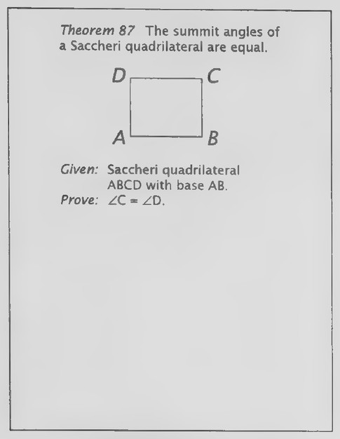Transparency 16-3-3: Theorem 87 (Lesson 2: Set I, Exs. 7-13)

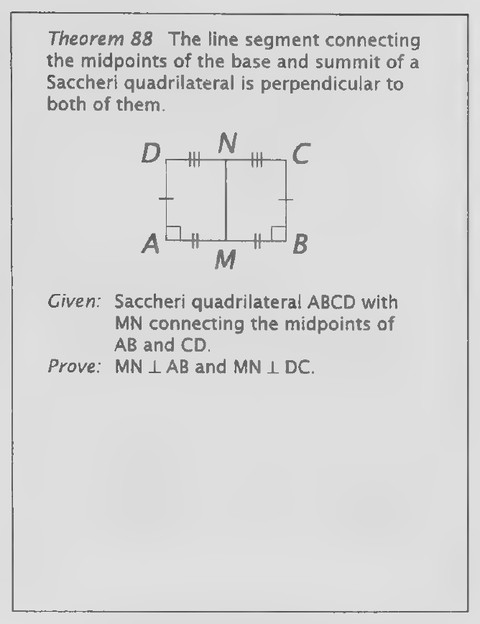Transparency 16-3-4: Theorem 88 (Lesson 2: Set II, Exs. 31-35)

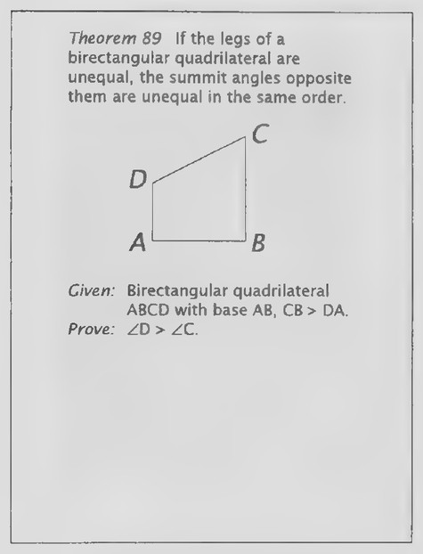Transparency 16-3-5: Theorem 89 (Lesson 2: Set I, Exs. 14-21)

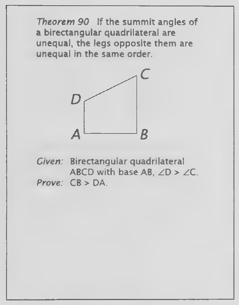Transparency 16-3-6: Theorem 90 (Lesson 2: Set I, Exs. 22-28)

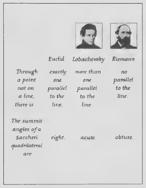Transparency 16-3-7: Table: Comparing three geometries

Saccheri quadrilateral are acute. We will refer to this as the “Lobachevskian Postulate” and we will use it to prove some theorems in Lobachevskian geometry. Although the proofs of the two theorems in this lesson are outlined in the exercises, I recommend considering the proof of Theorem 1 in class.

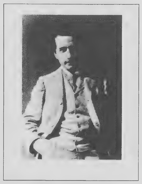Transparency 16-4-1: Photograph of Einstein

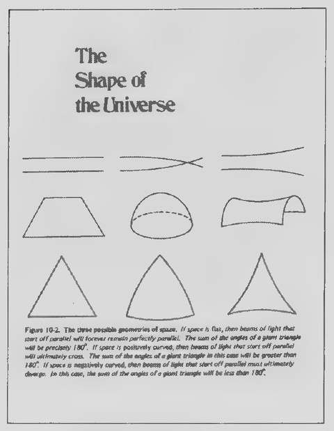Transparency 16-4-2: The shape of the universe

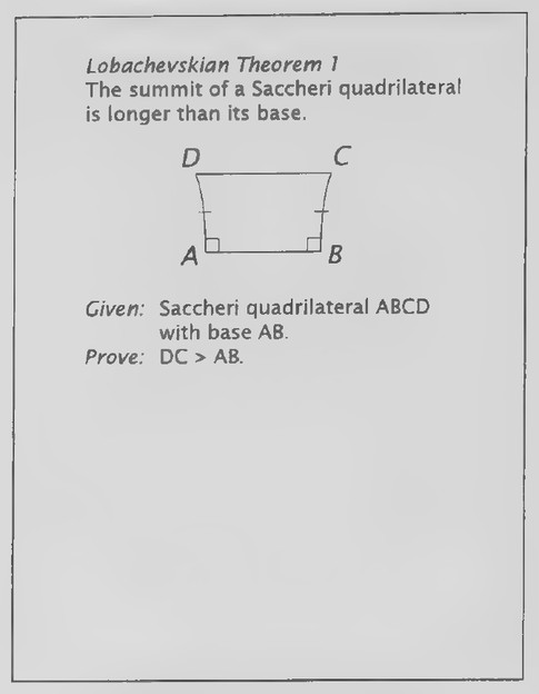Transparency 16-4-3

Lesson 4: The Triangle Angle Sum Theorem Revisited

Lesson Outline

Lobachevskian Theorem 3. The sum of the angles of

a triangle is less than 180°.

Corollary. The sum of the angles of a quadrilateral

is less than 360°.

Lobachevskian Theorem 4. If two triangles are

similar, they must also be congruent.

Transparencies

• 16-4-1 Photograph of Einstein
• 16-4-2 The shape of the universe 16-4-3. Lobachevskian Theorem 1 (Lesson 3: Set

I, Exs. 1-10) 16-4-4 Lobachevskian Theorem 2 (Lesson 3: Set

I, Exs. 11-18)

Introduction

The photograph of Einstein on Transparency 16-4-1 was taken when he was in his early twenties, not long before he developed the theory of relativity for which he was become so famous. Einstein once wrote that if he had not been acquainted with non- Euclidean geometry, he never would have been able to develop the theory of relativity.

The figures on Transparency 16-4-2 are from a book titled Relativity and Cosmology² and illustrate three possible geometries of space. (Read the caption to the figure.) From the standpoint of mathematics, all three geometries are equally valid. It

makes no sense to say that one of them is true and the others are false. If we are interested in deciding what the universe is like, then it does make sense to ask which geometry fits it. The theory of relativity implies that it may be one of the non-Euclidean geometries.

Transparencies 16-4-3 and 16-4-4 are for use in reviewing the proofs of the Lobachevskian Theorems 1 and 2. Again, even though the proofs of the theorems in the new lesson are outlined in the exercises, it may be best to preview at least one of them in class.

Review of Chapter 16

Transparencies

• 16-R-1 The orbit of Mercury
• 16-R-2 Lobachevskian Theorem 3 (Lesson 4: Set

I, Exs. 1-9) 16-R-3 Corollary (Lesson 4: Set I, Exs. 10-13) 16-R-4 Lobachevskian Theorem 4 (Lesson 4: Set

I, Exs. 14-20) 16-R-5 McDonald’s restaurants around Kansas

City 16-R-6 Point distributions on a plane and on a

sphere 16-R-7_ Escher’s Circle Limit III and diagram

First day

Introduction

Sir Isaac Newton, one of the greatest scientists of all time, was strongly influenced by Euclid. Of his books, the Principia, which is modeled after Euclid’s Elements, the Encyclopaedia Britannica says:

*Relativity and Cosmology by William J. Kaufmann III (Harper and Row, 1973).

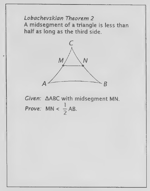Transparency 16-4-4: Lobachevskian Theorem 2 (Lesson 3: Set

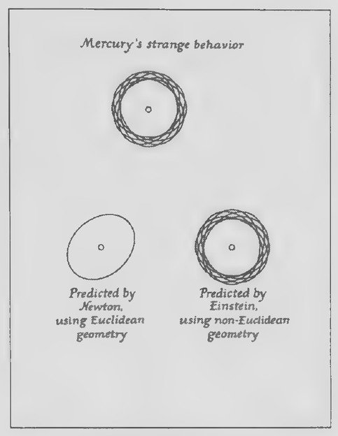Transparency 16-R-1: The orbit of Mercury

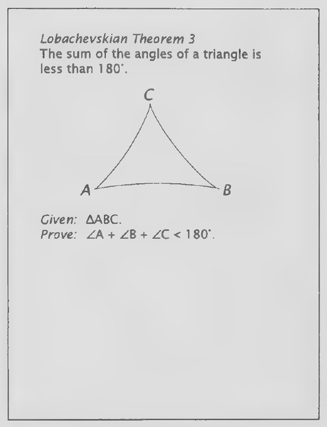Transparency 16-R-2: Lobachevskian Theorem 3 (Lesson 4: Set

It is explained for the first time the way in which a single mathematical law could account for phenomena of the heavens, the tides, and the motions of objects on the earth. The whole development of modern science begins with this great book.

The Principia was published in 1687. One hundred fifty years later, a French astronomer made a surprising discovery about the planet Mercury. Show the top figure on Transparency 16-R-1. This figure, greatly exaggerated to make it easier to see, represents the orbit of Mercury about the sun. In the course of each revolution, the orbit shifts very slightly. This is strange because, according to Newton’s laws of gravity, Mercury’s orbit shouldn’t do this. Show the lower-left figure on the transparency. The orbit should be a simple ellipse that remains fixed in space. Instead, it rotates very slowly, by about 43 seconds of arc each century.

In 1915, Einstein figured out why. Read the following passages, which are from Chapter 8 of Einstein: The Life and Times by Ronald W. Clark:

… Thus the universe which Newton has seen, and for which he had constructed his apparently impeccable mechanical laws, was not the real universe but only what he had seen through the misleading spectacles produced by gravity. The law which appeared to have worked out so well had been drawn up for a universe that did not exist, as though a tailor had made a suit for a man he had seen only ina distorting mirror..

Einstein’s paper gave not only a corrected

picture of the universe but also a fresh set of mathematical laws by which its details could be described…. These laws utilized Riemannian geometry, the need for which had been the direct result of the assumption that light would be deflected by a gravitational field and that the shortest distance between two points in such a field would not, when viewed from outside it, be coincident with a straight line..

Einstein had seen that his assumption of a curvature of light in a gravitational field meant that Euclidean geometry, satisfactory enough when coping with the small distances of everyday life, had to be replaced by something more sophisticated when dealing with the universe..

Einstein used Riemannian geometry to create equations by which the movements of the stars in their courses and the structure of the universe itself could be described…*

Show the lower-right figure on Transparency 16-R-1. Whereas Newton’s theory of the universe, based on Euclidean geometry, predicts an orbit for Mercury that does not match its actual path, Einstein’s theory, based on Riemannian geometry, predicts it perfectly. According to Einstein, the orbit should rotate 43 seconds of arc each century—the very amount that it does!

Because of this and other evidence, Einstein’s theory of relativity is generally accepted as correctly

*From Einstein: The Life and Times by Ronald W. Clark. Copyright © 1971 by Ronald W. Clark, with the permission of Thomas Y. Crowell Company, Inc., publisher, and The Harold Matson Company, Inc.

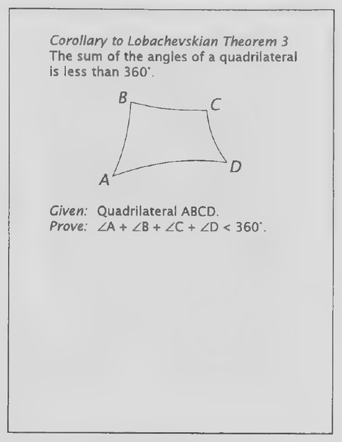Transparency 16-R-3: Corollary (Lesson 4: Set I, Exs. 10-13)

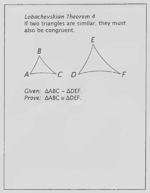Transparency 16-R-4: Lobachevskian Theorem 4 (Lesson 4: Set

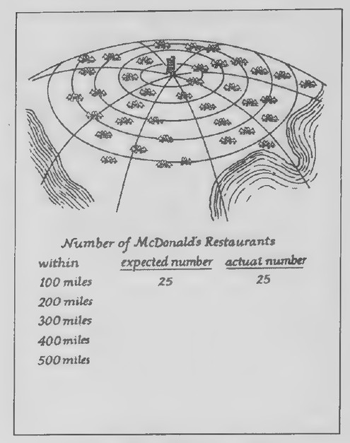Transparency 16-R-5: McDonald’s restaurants around Kansas

explaining the nature of the universe. It is amazing to think that it is based on a geometry that is non- Euclidean.

Transparencies 16-R-2, 16-R-3, and 16-R-4 are for use in reviewing the proofs of the theorems in Lesson 4.

First day

Introduction

The first McDonald’s hamburger stand opened in 1940 and since then thousands of McDonald’s restaurants have opened in the United States.* Suppose that the president of McDonald’s wanted to find out how the restaurants are distributed through the country. Show Transparency 16-R-5. He might choose a point in the center of the United States—say Kansas City—and decide to count the number of restaurants within 100 miles from this point, 200 miles from it, 300 miles from it, and so on.

Suppose that there are 25 McDonald’s restaurants within 100 miles of Kansas City. If the restaurants are distributed uniformly throughout the country, how many would you expect to find within 200 miles of Kansas City? Because the area of a circle varies as the square of its radius, it would seem that there should be four times as many restaurants in the circle whose radius is twice as large. Within 300 miles of Kansas City, we might expect nine times as many restaurants, and so on. Complete the expected-number column at the bottom of the trans-

parency. The numbers are: 25, 100, 225, 400, and 625.

Now suppose that the actual numbers of restaurants turn out to be as shown here. (Add the overlay.) We see that, as we get further and further from Kansas City, the actual numbers of restaurants fall further and further behind what we had expected. Does this mean that the restaurants are not uniformly distributed but are concentrated around Kansas City?

The answer is no! Our calculations were based on the assumption that the earth’s surface is flat, but it is not. It is curved. Show Transparency 16-R-6. These figures represent the sets of points within 1, 2, 3,4, and 5 units from a given point ina plane and on a sphere. The relations of the areas of the circles on the plane are what we assumed in predicting the numbers of McDonald’s restaurants at various distances from Kansas City. The areas of a comparable set of circle on the sphere have a different relation. As their radii increase, their areas do not grow quite as fast. This explains how the restaurants could be uniformly distributed and yet fall short of the numbers we predicted.*

The point to be learned from this story is that, if we assume that something is uniformly distributed over a surface, we can determine whether the surface is flat (Euclidean) or curved (non-Euclidean) by measuring numbers of the thing at varying distances from a given point in the surface. This is one of the methods astronomers have used to try to de-

‘The decline in “actual” numbers of McDonald’s restaurants in the table on the overlay to Transparency 16-R-6 is actually highly exaggerated to make the point more obvious.

*This story is adapted from one by George Gamow in his book, Mr. Tompkins in Paperback (Cambridge University Press, 1965).

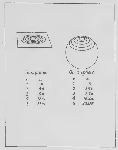Transparency 16-R-6: Point distributions on a plane and on a sphere

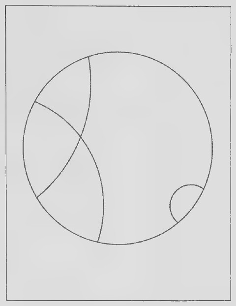Transparency 16-R-7

termine whether physical space is Euclidean or non- Euclidean. Although the problem is now three-dimensional rather than two-dimensional, the principle is the same.

In a survey of radio sources in space, astronomers at Ohio State University discovered that the farther out in space one looks, the more the number of observed radio sources falls short of what one would expect if space were Euclidean.* If we assume that radio sources are uniformly distributed throughout space, one implication that can be drawn is that space is non-Euclidean in nature. This, as you may remember, is in agreement with Einstein’s theory of relativity.

It would be interesting to know, if there are other intelligent civilizations in the universe, whether they also began with Euclidean geometry as we did. Of course they would call it by a different name. Because, on a small scale, Euclidean geometry seems so obvious, this seems very probable.

It would also be interesting to know how long it took them to realize that there are other geometries which might fit physical space instead. It took mankind two thousand years to do so!

Transparency 16-R-7 and its overlay are for use in discussing Poincaré’s model of Lobachevskian geometry. Show it first with the overlay in place and then remove the overlay to review the idea of orthogonal circles. Escher was inspired to create Circle Limit IITin 1959 as the result of correspondence with the geometer H. S. M. Coxeter.

*From Relativity and Cosmology by William J. Kaufmann III (Harper and Row, 1973), pages 112-113.

Notes on the chapters

About GEOMETRY by Harold R. Jacobs

Notes by Peter Renz

Geometry is intuitive and appealing with useful results but it can be demanding, and it has tricky twists and turns. The challenge is to build intuition and develop. the curiosity and persistence needed to push through tough problems and avoid pitfalls. Working with Jacobs on this book was a chance to fit the pieces of geometry into a coherent whole.

Particular examples are the core of this book, especially those in its exercises, as Don Albers notes in his Foreword. Every chapter offers a new crop of puzzles and applications. By following the steps of the exercises, you can always see what is happening, but in seeing why may be a challenge.

As I struggled, I remembered the NCTM Standards recommendations about flexibility. Use the tools best suited to a particular problem; choose your approach — direct geometric arguments, transformations, matrices, graphs, technology, whatever. This is fine advice for me, but the students are just starting out. Many times I found an easy approach but sometimes there were difficulties. Perhaps you will find the Royal Road I missed.

Euclidean geometry can be regarded as a system developed from postulates or as the geometry of the coordinate plane with the usual distance formula. Either way, the same properties hold. These properties are built into geometric software; they underlie computer representations, three-dimensional graphics, etc. If students understand that things must fit together, they will be able to check ideas for correctness using whatever tools are at hand — starting with paper, pencil, and brain power.

My experience is that looking things up and asking others for ideas are excellent problem-solving techniques. But nothing beats knowing the answer from school. A reasonable repertoire of standard results and formulas is useful, which is one reason a Formulary was added in this edition.

These notes outline key and motivating ideas for students and provide background for teachers, as well as outlining how to crack some tough nuts for those who want to prove some of the conjectures arising from the exercises.

Reading Geometry or teaching from it, you are bound to find questions and answers not touched on in these notes or in Jacobs’s Teacher’s Guide. Harold Jacobs and I would be happy to read your comments and suggestions and to try and answer any questions you may have. We can be reached care of W. H. Freeman and Company by mail or electronically.

Peter Renz

©2003 Peter L. Renz Used by permission.

Notes — Chapter 1: An Introduction to Geometry

To the Student. Your study of geometry builds on intuitive understandings: for example, of how rulers are used and of how braces can steady a framework. Geometry gives you tools for systematically solving problems such as those of the Surfer and Spotter. This chapter shows how problem-solving led to the development of geometry and how geometry, in turn, helps solve problems. Here we first meet the geometric terms and ideas that are used throughout the text.

The final lesson, We Can’t Go on Like This, shows the need for a more systematic approach. In geometry examples let you see what is going on — what works and what doesn’t. But you need tools to help you discover things, to avoid fooling yourself, and to back up your insights. These you will master as you work through this book. Revisit the Surfer, the Spotter, and other problems. You will find simpler approaches and new understandings as you move ahead. _

Lesson 1. Lines in Designing a City. The terms point, line, line segment, and plane are informally introduced, followed by definitions of several terms relating these basic geometric concepts: collinear and noncollinear, coplanar, and concurrent.

Interesting configurations of lines are included in the exercises. Students are asked to look at figures, identify and count their components, and draw other figures that lead to results that are both puzzling and surprising. These teach the basics and will suggest a world of possibilities to the student whose curiosity is aroused.

Lesson 2. Angles in Measuring the Earth. The terms ray and angle are informally introduced and the use of a protractor to measure angles is reviewed.

The exercises ask the students to make visual judgments followed by practice in making accurate measurements to verify them.

Lesson 3. Polygons and Polyhedra: Pyramid Architecture. The terms polygon and polyhedron are informally introduced, together with the names of the most commonly encountered polygons. The concepts of perimeter and area are reviewed.

The exercises range from questions about pentominoes to building a model of the Great Pyramid to a remarkable dissection problem (for the latter see also under Set III of Lesson 1, Chapter 7).

Lesson 4. Constructions: Telling Time with Shadows. The idea of a construction is introduced and the methods for carrying out two basic constructions, bisecting a line segment and bisecting an angle, are introduced without proof.

In the exercises, constructions are applied to finding north with shadows, determining the hour spokes of

a simple sundial, and discovering something surprising about bisecting the angles of a rectangle.

Lesson 5. We Can’t Go on Like This. The concluding lesson of this chapter emphasizes that our thus-far informal approach to geometry has led to interesting as well as practical results but is ultimately unsatisfactory because we have no convincing basis for knowing that the conclusions we have been drawing are necessarily correct.

The exercises show the need for critical thinking and careful analysis. They are also provocative: Why is it easy to trisect a line segment, yet impossible to trisect an angle with only straightedge and compass? Why do several consecutive figures showing regions formed in circles seem to establish a simple pattern, after which the pattern fails?

Notes — Chapter 2: Deductive Reasoning

To the Student. Chapter 1 showed geometry being used in many ways over the ages but concluded “We can’t go on like this.” Then how to proceed? The answer is: “Deductively and carefully.” Euclid showed the way around 300 B.C., and there have been many additions and improvements since. He gave us geometry as a deductive system, with clear assumptions (the postulates), definitions, and methods for proving what is true, our theorems.

You already know how to make deductions. If you look out the window and see rain, you deduce that there are clouds in the sky, even if you can’t see the sky from your window. Deductive reasoning is the stuff detectives use; it can help you solve puzzles and solve problems. We end this chapter with some famous theorems of geometry, some of which you probably know already. As we work through the course, you will see why these must be true and how they can be proved.

Lesson 1. Conditional Statements. These are the basic tools of deduction. Using Agatha Christie’s detective Hercule Poirot, we introduce such statements and the ways they are represented symbolically and by Euler diagrams. The examples and exercises give students practice in interpreting these forms and moving between them.

Lesson 2. Definitions. In formal arguments, we often need to replace a reference to some property or thing with the definition of that property or thing, so this chapter covers definitions, the converses of conditionals, and logical equivalence. The symbolic forms a — b, a <— b, and a + a, as well as the abbreviation “a iff b” are covered. The examples and exercises give practice in recognizing and shifting between these various representations.

Lesson 3. Direct Proof. This workhorse of deduction is introduced by a Rube Goldberg cartoon. The

symbolic and Euler diagram interpretations reinforce the idea behind this valid form of inference. Exercises show that direct proof is an effective tool for critical thinking and for solving puzzles and problems.

Lesson 4. Indirect Proof. If assuming the opposite (or logical negation) of your desired conclusion leads to a contradiction, then your desired conclusion must be true. Examples given of this basic method of proof range from concluding that an ammonia molecule cannot be planar, to analyzing possible poker hands, to coin-weighing problems.

Lesson 5. A Deductive System. To avoid circularity or infinite regress, some terms must be taken as basic and left undefined; certain observations must be taken as postulates. With postulates, definitions, and means for dzrect and indirect proof to derive our theorems, we have the basis for the deductive system we use in the study of geometry.

This lesson includes our first two postulates. Postulate 1: Two points determine a line. Postulate 2: Three noncollinear points determine a plane. Note that “two points” should be understood as meaning the same as the alternative “two distinct points.” Either form is acceptable, but the former is simpler and agrees more closely with common usage.

Lesson 6. Some Famous Theorems of Geometry. An opening “B.C.”cartoon makes the point that many students will already know results such as the a? + b? = c? of the Pythagorean Theorem and the fact that the sum of the angles in a triangle is 180°. Jacobs takes advantage of this head start and brings other students up to speed by introducing these results along with Circumference = 2ar and Area = mr? for the circle. He gives plausibility arguments for the Pythagorean Theorem and the Angle Sum Formula for triangles and discusses the results for the circle, leaving proofs for later.

Using these results, students can do applied problems that provide practice with algebraic methods, as the exercises show.

Looking Ahead. We prove the Angle Sum Formula for triangles using the Parallel Postulate in Chapter 6. We offer two approaches to the Pythagorean Theorem: one via areas (the formal version of the plausibility argument given in this chapter) and the other by similar triangles (Chapter 11, Lesson 2). The later approach uses the Angle Sum Theorem. For the circumference and area of the circle we use a limiting argument, like the method of exhaustion used by Archimedes (Chapter 14 of Geometry and in these notes).

Notes — Chapter 3: Lines and Angles

To the Student. Intersecting pairs of lines form angles, and pairs of points define segments. We measure angles in degrees and intervals by their lengths, using various units. When you compare equal segments using a ruler, you could as well have copied the first segment onto the edge of the ruler and moved that copy over the other segment, matching it exactly. This matching is geometric equality, called congruence. A protractor lets you compare angles in the same way.

We begin with the algebraic tools used in geometry. Next come the Ruler and Protractor Postulates and the ideas about measuring distances and angles sketched above. We will cover complementary and supplementary angles, linear pairs, vertical angles, perpendicular and parallel lines, among other ideas. _ “

Lesson 1. Number Operations and Equality. This covers the transitive property of equality and “common notions of Euclid” such as “If equals be added to equals, the results will be equal.” These are part of algebra, and students will have seen them, but possibly in different forms. Here they are, with examples of their geometric uses. This lesson is an anchor for the algebra strand in this book. An algebraic puzzle from Lewis Carroll wraps up the lesson.

Lesson 2. The Ruler and Distance. Numbers and algebra do much of the work in our geometry. To move ahead we need the Ruler Postulate and the betweenness of points properties of this lesson. We have the theorem: If B lies between A and C on line /, then AB + BC = AC. The converse of this theorem follows from the triangle inequality: AB + BC > AC, unless B lies in the interval from A to B. We will prove this Chapter 5, on inequalities.

Lesson 3. The Protractor and Angle Measure. The Protractor Postulate does for angles what the Ruler Postulate did for the lengths of segments. There is no natural scale for lengths, but a half-rotation and a right angle are natural units for angles. When Euclid stated his Fourth Postulate, “All right angles are equal,” he was stating that angles that have the same measures in terms of halves or quarters of a circle are geometrically the same (congruent). Set III introduces the Tantalus problem. The key to the Tantalus problem lies in the figure for the Angles Problem on page 515.

Lesson 4. Bisection. Rulers and protractors allow us to divide segments or angles into any desired proportions. Such division can be done using algebra, with a calculator or computer software to carry out the details. Geometrical bisection is based on congruence, as we will see in Chapter 4. It also brings in ideas of reflection and symmetry that we will revisit in Chapter 5. A fold, not a ruler, gives you the quickest way to divide a piece of paper in half. Applications include origami, molecular

structures, carpentry, and the shapes of flowers. This lesson and its exercises revisit earlier ideas, including measurement, the use of coordinates, and constructions.

Lesson 5. Complementary and Supplementary Angles. These ideas are algebraic. Angles A and B are complementary if A+B = 90°, they are supplementary if A +B = 180°. Angles supplementary (or complementary) to the same angle are equal. The exercises give practice in algebra, logical reasoning, and seeing geometric configurations.

Lesson 6. Linear Pairs and Vertical Angles. Linear pairs are a natural geometric setting for applying the ideas of supplementary angles. The Protractor Postulate lets us prove that vertical angles are equal using algebra. Similar reasoning is used in the exercises to work out angles in folding chairs and in garden shears. In Set III, students figure out a proof from a Chinese geometry book.

Lesson 7. Perpendicular and Parallel Lines. Here we encounter two key concepts. If one of the four angles formed by intersecting lines is a right angle, then the lines are perpendicular and all four angles are right angles. Parallel lines lines lie in the same plane but do not intersect. Already, students should have the idea that parallel lines have the same direction. Indeed, this is what the Parallel Postulate of Chapter 6 will tell us.

Notes — Chapter 4: Congruent Triangles

To the Student. Congruent triangles have the same size and shape. We begin our study of shapes with them. You will see how their shapes are determined by lengths of sides and sizes of angles. Shapes can also be described using coordinates, as you will see in the first lesson of this chapter. The distance and angle approach of congruence and the coordinate approach work together. Surveyors work out coordinates using distances and angles, and you will see that the Pythagorean Theorem lets you find distances from coordinates.

Key concepts in this chapter are: coordinates and the distance formula (use of the Pythagorean Theorem), and congruence and the ways to prove that triangles are congruent. Key techniques are: using coordinates to describe shapes and find distances, using and marking diagrams to show geometric relationships, and showing that triangles are congruent so that various segments and angles must be equal.

Lesson 1. Coordinates and Distances. Maps motivate the idea of a rectangular coordinate system and its coordinate grid. The Ruler Postulate gives us the numbers on the axes. The Pythagorean Theorem (Chapter 2, Lesson 6) gives us the distance formula. Examples in the exercises include the Geoboard, map reading, optics, plots of characteristics of birds and bats, architecture, and computer displays. The vector picture is introduced using water velocities.

Lesson 2. Polygons and Congruence. Congruence is the key idea here. Trace a polygon, if the tracing can be set down on another polygon so the two coincide then they are congruent. The lengths of corresponding segments and the sizes of corresponding angles must be equal. For triangles, the equality of corresponding parts defines congruence. Later, we will relate congruence to isometries. Examples used in the exercises include: a connect-the-dot figure, a patent drawing, an “art gallery” problem, and a fractal curve. There are many discovery exercises, and there is much practice with coordinates.

Lesson 3. ASA and SAS Congruence. A dramatic application of the ASA method from World War II opens the lesson. The lesson shows why the ASA and SAS Congruence Postulates should be true. The exercises show how useful these postulates are. Key terms such as included angles and opposite sides are defined. An exercise anticipates the names of types of triangles that will be formally given in Lesson 5. Applications include: binocular vision, measuring the Earth, and surveying.

Lesson 4. Congruence Proofs. A cartoon introduces a use of the ASA Postulate. A paragraph proof leads students to a second two-column proof. A discussion follows of the various ways proofs can be written. Applications are given to roof construction and estimating distances. There is practice bringing coordinate and congruence ideas together. There are exercises involving overlying triangles by folding paper that bring home the physical meaning of congruence.

Lesson 5. Isosceles and Equilateral Triangles. If two sides of a triangle are equal, the angles opposite them are equal. Jacobs presents Pappus’ beautiful proof of this result. He avoids “base angles” to let students think more easily of these triangles in various orientations. This lesson has a rich harvest of theorems and corollaries, and the exercises offer practice with proofs.

An application to the geometry of the hydrogen sulfide molecule is worth mention. This atom has a bond angle of 92.8°. The Pythagorean Theorem does not apply directly, but as an approximation it is good to within 2%. An Escher tiling is the Set III puzzler, where a mirror-image piece provides a final twist.

Lesson 6. SSS Congruence. Seeing that triangular braces make frameworks rigid motivates introduction of the powerful SSS congruence theorem. Jacobs gives Euclid’s proof.

Exercises include showing why the bisection constructions from Chapter 1 work.

A cautionary exercise shows that two triangles can have five pairs of parts equal and not be congruent. The geometry of linkages and of the plumb level is examined in the exercises. Vectors appear as forces that are in

balance if when arranged head to tail they form a triangle. Identifying types of triangles given in coordinate form gives practice with the use of coordinates and the distance formula.

Lesson 7. Constructions. Methods for copying segments, angles, and triangles complete our list of basic straightedge and compass constructions. Walk your compass down a line marking equal segments and you have the start of a ruler. Add in marks for halves, quarters, and so on by bisections, and you can pin down the coordinates of points as closely as you wish. Such constructions are background for the rulers, protractors, and coordinate systems of metric geometry — and they show how distances and shapes are determined by lengths and angles.

The exercises give a striking example of a construction discovered in 1743 in Sweden for determining where the frets go on a guitar, still a tricky problem. In making this construction, we use a ruler to shorten the work of making equal divisions on a base line. Other examples in the exercises include girders, jacks, and the reflection of light.

Notes — Chapter 5: Inequalities

To the Student. Geometric inequalities spring from this fact: The whole is greater than the part. For example, we show that the angle opposite the smaller of two sides in a triangle is congruent to a part of the angle opposite the larger side. This gives a theorem: If two sides are unequal in a triangle, the angles opposite to them are unequal in the same order. Congruence, the whole-part relationship, and the algebraic properties that begin the chapter will be important tools throughout it. When direct comparison of A and Z is difficult, a convenient intermediate quantity, say X, can often be found so that you can show A < X and X < Z. Then, you can conclude A < Z using the transitive property of inequality. Watch for this technique.

The changes in appearance as a configuration shifts or is seen from different points of view are a theme in this chapter, starting with a description of experiments on an infant’s sense relative distance and ending with Galileo’s observations of the planet Venus. The Triangle Inequality lets us work out the possibilities for the distances Galileo wondered about. These are consistent with the range of apparent sizes for Venus in its various phases. Art and architecture are concerned with the effects of changes in point of view and many examples in this chapter are drawn from these fields. In addition, you will see applications to planning kitchens and designing mechanical devices. _ til

Lesson 1. Properties of Inequality. This lesson opens discussing experiments that showed that depth perception is inborn. This leads to the algebraic properties of inequality, part of the algebra strand of this

book. The sum of positive numbers is greater than any of its summands. For Euclid this was again: the whole as greater than the part. The phrasing suggests a key idea of this chapter. Transitivity plays an equal role, as well. The other algebraic properties of inequalities. are needed for working out the consequences of various geometric conditions.

Visual effects and illusions are a theme in this chapter. Students draw figures, measure, and discover relationships that will be proven later. Applications include art and architecture.

Lesson 2. The Exterior Angle Theorem. A hoyering U. F. O. is sighted from two points on the ground giving a triangle whose geometry shifts as the U. F. O. moves. We see one relationship that seems to hold in this triangle whatever shape it has: The exterior angle as larger than either remote interior angle. Jacobs gives Euclid’s proof using congruence and the relationship of the whole to a part.

Applications in the exercises include scale drawing, measurement, and mechanical devices. In the exercises, students extend the argument given in the text to deal with the other remote angle, and they see an alternative proof of the Exterior Angle Theorem devised by Proclus.

Lesson 3. Triangle Side and Angle Inequalities. The opening painting shows how a change in point of view can dramatically alter appearances. As in Lesson 2, we see that certain geometric relationships must hold no matter how the scene is viewed.

If a triangle has unequal angles the opposite sides will be unequal in the same order. This gives the qualitative relationship between angles of a triangle and their opposite sides. The quantitative relationship is given by the Law of Sines, which appears in the lessons on trigonometry in Chapter 10, The Right Triangle.

There is opportunity for a good deal of critical thinking in the exercises. Set II begins with a discovery exercise leading to an alternative proof of the main result of this lesson. The last exercise in Set II revisits the Surfer problem from the book’s Prelude.

Lesson 4. The Triangle Inequality Theorem. The final lesson of this chapter, like the initial lesson is concerned with the perception of distance. This time we begin with Galileo’s speculations on the distance to the planet Venus. This lesson opens with five pictures of the planet Venus at various phases all shown at the same scale. The smallest disk, the full phase, is about a sixth the diameter of the new phase, the largest of these images. The geometry of the Venus, Sun, Earth system gives a triangle and the variations of that triangle motivate our discussion of the Triangle Inequality: The sum of two sides of a triangle exceeds the length of the third.

Exercises are based on examples from planetary motion, optics, and kitchen design, with the Surfer of the Prelude appearing as well.

In Euclid’s time people objected that the Triangle Inequality was obvious and did not require proof. But the interest in this theorem lies not in the fact that it is true, but in why it is true — and in the consequences we can derive from it. Using it and some basic distances, we see that Venus at its most distant point (in its full phase) is over six times the distance it was from Earth at its closest approach (in its new phase). This suggests why Venus in its full phase has an apparent size about a sixth of that of its full phase, as our pictures show.

The working out of the sizes of the orbits of the planets is a difficult technical matter. The underlying principle that we see here is that all of the measurements and observations must form a consistent picture. The variations in the apparent diameter of Venus in its various phases fit with the orbital sizes we give. Apparent diameters are measured in degrees or radians and the rough inverse proportionality to distance observed here should be expected. The reason is that, for small angles, the angle measure, the sine, and the tangent are all close to being proportional.

ll” Lines Are Determined by Distances. A corollary of the Triangle Inequality Theorem is that for three noncollinear points AB + BC > AC, so B can not satisfy the metric condition for being between A and C. Consequently, if AB + BC = AC, then B must lie on the same line determined by A and C, and B must be between A and C on that line. If we know the distances between all pairs of points, we can tell which points are collinear and which points lie between any given pair of points. Euclidean geometry can be developed using ideas of distance alone, although this approach is neither as easy nor as intuitive as ours. See, for example, Leonard M. Blumenthal’s book A Modern View of Geometry, W. H. Freeman and Company, San Francisco, 1961. _

▶ About Estimation. Inequalities are often used in estimation. For example, Archimedes trapped the circumference of a circle of diameter d = 1 between the perimeters of inscribed and circumscribed regular polygons of 6 x 24 = 96 sides. Using these perimeters, he showed that the circumference of this circle, πd = m1 = 7, lay between 370 and 3. In short, he proved that 37° yi RES 3. This was a considerable achievement for Archimedes, although a student with a scientific calculator can whip out the equivalent result in decimal form in a few minutes. That’s progress. We also have progress in estimation of 7, which is now known to an accuracy of billions of decimal places, although not by finding the perimeters of regular polygons. (See Supplemental notes for Chapter 14 for Archimedes’ calculation and see “to calculate better” in the supplemental material for Chapter 11 for high-precision 7 calculations.)

Precision calculations come with error estimates that are worked out using basic properties of inequalities.

For this reason, the study of inequalities is not a sideline, but is a central concern both for mathematics and for its applications. “

Notes — Chapter 6: Parallel Lines

To the Student. Lines are parallel if they lie in the same plane and don’t intersect. Parallel lines should have the same direction. In particular, through a point P not on a given line £ there should be exactly one line parallel to the line £. Why? Because through the point P there should be exactly one line ℓ’ having the same direction as line. The Parallel Postulate tells us there as exactly one such line ¢’. With the Parallel Postulate we can characterize parallel lines by the angles formed by lines cutting across them, transversal lines. We will also prove the Angle Sum Formula for triangles and establish the Angle Angle Side (AAS) and Hypotenuse Leg (HL) congruence theorems. _ “

Lesson 1. Line Symmetry. Paper folds, linkages, and symmetrical art and diagrams motivate the study of line symmetry in this lesson. Two points A and B are symmetric with respect to the line ¢ iff @ is the perpendicular bisector of the segment AB. The construction of perpendicular bisectors and the proof of the correctness of this procedure is background for the construction of parallels in the next lesson. It also sets the stage for the contrast made in Lesson 3 between the uniqueness of perpendiculars, which we can already prove, and the uniqueness of parallels, which can only be proved by introducing the Parallel Postulate. Line symmetry is treated as a property of figures. In Lesson 3 of Chapter 8, we will revisit line symmetry in terms of reflections and transformations.

The Set III exercise asks the students discover some properties of an amazing set of points in the plane. See the discussion given with Jacobs’s answers.

Lesson 2. Proving Lines Parallel. Parallel lines were defined earlier in Lesson 7 of Chapter 3. Here we see that the Exterior Angle Theorem allows us to conclude that two lines in a plane that make equal corresponding angles with a transversal cannot intersect. This gives us Theorem 17: Equal corresponding angles mean that lines are parallel. This statement is given in a simple and general form. Each application of this result requires students to think through the geometry and recognize the corresponding angles so that the basic idea and its uses are gone over repeatedly. The same is true for the corollaries given in this lesson. The exercises drive home these ideas. The converse of Theorem 17 is true, but its proof comes in Lesson 4 after the Parallel Postulate has been given in Lesson 3.

Lesson 3. The Parallel Postulate. Given a line é and a point P not on @ we know how to construct a line n through P parallel to. We also can construct an m which is perpendicular to @ and passes through P.

For perpendiculars, we can prove that there is exactly one such line m. This lesson asks the question: Can we prove that there is only one such line n, when n line is to be parallel to ℓ rather than perpendicular to ℓ2? The answer is: Not without a further assumption. This is further explored in Chapter 16, Non-Euclidean Geometries, but the assumption we need, the Parallel Postulate, is introduced here.

Set I. Exercises 11-18, Exactly One, focus on the meanings of “at least,” “no more than,” and “exactly.” Gateway (37-41) raises questions about what we know about figures and what is yet to be proven. Windshield wipers, gateways and paper folding are among the examples used in the exercises.

▶ About The Parallel Postulate. It took more than two thousand years for geometers to discover that the Parallel Postulate, or equivalent statements, could not be proven from the other axioms of Euclid’s system. The discovery of non-Euclidean geometries shook the faith people had in fixed systems of knowledge. The words of Morris Kline at the beginning of his chapter on non-Euclidean Geometries in Mathematical Thought from Ancient to Modern ‘Times, Oxford University Press, 1972, gives a sense of this. Kline wrote:

“Amidst all the complex and technical creations of the nineteenth century the most profound one, non- Euclidean geometry, was technically the simplest. This creation gave rise to important new branches of mathematics but its most significant implication is that it obliged mathematicians to revise radically their understanding of the nature of mathematics and its relation to the physical world.”

Where does this leave us? For one view, read the conclusion to Jan Gullberg’s section on non-Euclidean geometries in Mathematics: From the Birth of Numbers: “… Euclidean geometry is still the basis for most practical applications of geometry — it has taken human beings to the Moon and beyond.”

Lesson 4. Parallel Lines and Angles. The naturalist Jean Henri Fabre’s analysis of the geometry of a spider’s web leads in to this lesson on the converses of Theorem 17 and its corollaries. Now that we have the Parallel Postulate these converses can be proven. This lesson provides a natural opportunity to go over the distinction between a statement and its converse, both in the text and exercises.

The exercises include: proving that parallel lines are everywhere equidistant, an anticipation of the proof of the Angle Sum Theorem for triangles, and an exploration of the methods Kepler used in working out the path of Mars.

Lesson 5. The Angles of a Triangle. Over distances that are short compared to the earth’s radius, the sum of the angles in a survey triangle will be 180°. This is used as a check for measurement errors. This

idea opens our lesson. We prove the Angle Sum Theorem for triangles — a result announced in Lesson 6 of Chapter 2. We also prove Theorem 21: An exterior angle of a triangle is equal to the sum of the remote interior angles. This is a strengthening of Theorem 12, the. Exterior Angle Theorem found in Lesson 2 of Chapter 5. Useful corollaries include: If two angles of a triangle are equal to two angles of another triangle, then angles of the third pair are also equal and The acute angles of a right triangle are complementary.

The exercises include proofs of the corollaries in the lesson and an explanation of how the latitude of a town in the northern hemisphere can be determined by sighting the North Star.

Lesson 6. AAS and HL Congruence. A fractal construction using triangles introduces two new methods for proving that two triangles are congruent: the Angle Angle Side method (AAS, Theorem 22) and the Hypotenuse Leg method for right triangles (HL, Theorem 23). The proofs are immediate consequences of the Angle Sum Theorem of Lesson 5. This lesson gives an opportunity to review the methods of showing triangles congruent and to consider the questions of how many parts of two triangles can be equal without the triangles being congruent. This problem was looked at in the exercises for Lesson 6, SSS Congruence, of Chapter 4.

Set I. Triangle Problem (18-22) shows that a triangle is isosceles if its altitudes are equal. The Set II exercises begin by establishing the properties of mirror images, and Set III unveils the deceptions of the fallacious proof that all triangles are isosceles.

Notes — Chapter 7: Quadrilaterals

To the Student. ‘This page is rectangular, so are the doors you walk through and the floors you walk on. Rectangles, squares, parallelograms, and other quadrilaterals are found everywhere. In this chapter you will see that what you know about triangles and parallel lines will let you understand the geometry of quadrilaterals. Squares, rhombuses, parallelograms, and other quadrilaterals are used to design buildings and machines and in art. The chapter is organized around the types of quadrilaterals and their properties.

The dozen theorems in the body of this chapter catalog various sorts of quadrilaterals and the properties they must have. For your overview of this chapter, run through the types of quadrilaterals, drawing pictures of each type and reviewing its properties. The final lesson of the chapter gives you a new result about triangles that can be proven using what you have just learned. This result is the Midsegment Theorem, which tells you that the segment joining the midpoints of two sides of a triangle is parallel to and half the length of the third side. t

Lesson 1. Quadrilaterals. The chapter opening is an unusual shape for a quadrilateral. Jacobs chose this to sharpen the student’s appreciation of what is common and what is unusual in quadrilaterals.

In Chapter 1, Lesson 3, Polygons and Polyhedra, we defined quadrilaterals. We return to quadrilaterals with the machinery needed to develop their properties. Learning to see and identify the various sorts of quadrilaterals and to instinctively know their properties is the key to this chapter.

First, we distinguish between convex polygons and concave ones. Second, we observe that the Angle Sum Theorem for triangles lets us conclude that the angle sum for quadrilaterals in 360°. Hence, an equiangular quadrilateral has four right angles. This gives us the rectangle, the most useful quadrilateral.

Notice the discovery exercises in Set I: Rectangles (16- 18), Rhombuses (19 and 20), Squares (20 and 21), and Parallelograms (23-25). Here students begin to learn the names of various special quadrilaterals, to recognize them, and to see what properties they have. See Set II, Gemstone Patterns (36-49) and Linkage Problems (52-55), which are also exploratory. The amazing dissection in the Set ITI exercise was seen before in Lesson 3 of Chapter 1. The dimensions and angles in this dissection can be worked out starting from the fact that the area of both figures must be the same. This might be suitable for motivated students: perhaps working as a team, using technology such as Geometer’s Sketchpad™, or looking material up in the library.

Lesson 2. Parallelograms and Point Symmetry. We define parallelograms in this lesson and develop their properties, including their point symmetry. In the next lesson we will look at converse results, seeing which sets of these properties imply that a quadrilateral is a parallelogram. We return to symmetry from the point of view of transformations in the next chapter.

Set I. Optical Illusions (4-10) involving parallelograms are seen here. The point symmetry of parallelograms is proven in Exercises 16-23. Set II exercises begin with the parallelogram law for the addition of vectors. The Set III problem asks students to determine the symmetries of playing cards.

Lesson 3. More on Parallelograms. Here we see that quadrilaterals whose opposite angles are equal are parallelograms and so on. The lesson opens with a powerful visual illusion based on a room in which seeming rectangles turn out to be trapezoids. Note the way algebra and geometry work together in this lesson and in its exercises.

Set II. Rope Trick (36-43) gives a beautiful African method for laying out the rectangular base for a house. Flexible Grid (47-55) is intriguing. A surprising construction using equilateral triangles is the basis for the Set III exercise. See Alternating Triangles on page 565

of Geometry, and see these notes for hints on how to proceed.

Lesson 4. Rectangles, Rhombuses, and Squares. These are the figures you encounter most frequently in construction. We know a great deal about quadrilaterals, and the student sees how this knowledge can be put to use. See especially Exercises 26-39, Checking a Wall, which walk the student through the practical aspects of measuring the sides and diagonals of a wall to see whether it is rectangular.

Lesson 5. Trapezoids. These are less constrained: exactly one pair of sides of a trapezoid is parallel. Structure remains, particularly for isosceles trapezoids, whose nonparallel sides are of equal length. Trapezoids show up Stepladders (34-42) and in geometric Trademark (9- 13). Set III features a surprising solution to a classic problem. This solution was found by high school student Andrew Miller, while he was was working from the First Edition of this book.

Lesson 6. The Midsegment Theorem. The segment connecting the midpoints of two sides of a triangle is called a midsegment, and it is parallel to the third side and half its length. This is a new fact about triangles that follows from methods developed in this chapter. The Midsegment Theorem anticipates some ideas related to similar triangles that will be developed in Chapter 10.

Set II. The three-dimensional models in Tetrahedra (37-41) are worth special attention. See the discussion of these in the Answer section. In Exercises 27−36, Midpoint Coordinates, students discover the relationship between the geometric and coordinate views of midpoints. Base Average (49-54) begins by asking the student what seems to be true. Then we see how the natural conjecture can be proved. Set III looks at a geometric progression of similar triangles and asks the student to estimate the sum of the lengths of all their sides. See the Answers for comments and links to other material in the book.

Notes — Chapter 8: Transformations

To the Student. Trace ashape onto a transparent sheet and see whether you can move the sheet so that the tracing matches a second shape. If you can, the shapes are congruent. ’The motion of the sheet gives a transformation of the plane. If the motion is a sliding of the sheet without turning, the transformation is a translation. If you could pin the sheet at one point and turn it to make the match, the transformation is a rotation about the pinned point, its center.

To match a left handprint with a right one, you must flip the sheet over. You would reverse it left-to-right about the symmetry line between the two handprints. The handprints are congruent, but they look different because each is a mirror image of the other. Flipping

the sheet has the same effect as reflecting one handprint through the line of symmetry between the two prints.

To show that a left footprint is congruent to the next right footprint, trace the left footprint, slide the sheet forward a pace, then flip it over. A flip is always needed when matching shapes that are mirror images. This slide and reflection gives a glide reflection.

Two shapes in the plane are congruent precisely if one can be carried onto the other by one of the transformations described above. These are the transformations that preserve size and shape in the plane, the isometries of the plane. This chapter shows you what these transformations are, how they are defined by reflections, and how they relate to symmetry.

▶ On Transformations. |The material in this chapter has only been studied systematically for about 150 years. The ideas are basic and can be grasped intuitively, but the details could fill a course by themselves. Jacobs’s approach in the text is intuitive. This note sketches the origins of the transformational approach, how it relates to coordinates, and how one would prove the facts seen in this chapter.

Before geometry became a science, people recognized that some pairs of different things had the same or similar shapes. If two shapes are the same, then we could move one on top of the other so that they would coincide. Euclid used this notion for figures; it is called superposition in older texts. Postulates give us conditions for triangles to be congruent, meaning they are superposible. A full appreciation superposition came only with the systematic use of transformations in geometry. This was launched 1872 by Felix Klein in a lecture referred to as “Kline’s Erlanger Programm.”

For Euclidean geometry, the key transformations are the zsometries, the transformations of the plane onto itself that preserve Euclidean distances. A physical model these isometries is given by tracing figures onto sheets to see whether you can make one figure match another.

We can imagine our transparent sheet extends as far as we wish, so the isometry that shows that two figures are congruent can be applied to other figures traced onto the same sheet. Before there were flexible transparent sheets, geometers had already classified the isometries of the plane and shown how these transformations can be produced by single reflections or combinations of two or three reflections. Knowing what the isometries are allows us to make precise the Euclidean idea of superposition and to define congruence for any pair of figures.

In this chapter the properties of isometries are developed geometrically. In the exercises, students discover how transformations affect the coordinates of the vertices of figures. More elaborate coordinate methods are used for applications such as computer graphics or map making, but the link between transformations and coordinates is already clear from these exercises. (See

Matrices and Computer Graphics in the supplemental notes for Chapter 12 here.)

Jocobs lets students discover what transformations tell us about congruence and symmetry. He omitted proofs, but many facts about isometries are easy to estab- ‘lish. For example, if an isometry carries △ABC onto AA’B’C’, then △ABC & AA‘B’’C’, by SSS, so ∠ABC = ∠A’B‘C’, by CPCTE. This proves that isometries preserve angles because they preserve distances. For convenience, Jacobs made “preserving angles” part of his definition of zsometry, but this property is a consequence of preserving distances.

The properties of reflections are also taken for granted here, but they are also easily proven. Intuition tells us that when A and B are reflected in line ℓ to give A’ and B’ we have equality of lengths: AB = A’B’. This follows from the definition of reflection and the congruence postulates. It is also intuitive that if two transformations both preserve distances, then their composition also preserves distances. Because of this, any composition of reflections is an isometry. Jacobs left this as an unstated assumption, but is easy to state and prove.

Isometries of the plane are either reflections, translations, rotations, or glide reflections — plus the unmentioned identity transformation. Each sort of isometry is characterized by certain properties. For instance, reflections leave just the points on their mirror line fixed and rotations leave only their centers fixed, except for rotations by multiples of 360°, which leave every point fixed. Translations by a positive distance move lines onto lines parallel to themselves and leave no point fixed.

Conversely, a 1:1 transformation of the plane onto itself that sends lines onto lines parallel to themselves and that leaves no point fixed must be a translation. Here is why: Pick a test point P, it moves to some other point P’. Look at the line PP’. The image of this line is parallel to the original line and contains P’, so this line is sent into itself. We say this line is znvariant. The same argument applies to any other point Q, so the line QQ’ is also invariant. If these lines were to intersect, their point of intersection would have to be a fixed point. Because our transformation has no fixed points, QQ’ ∥ PP’. Also, PQ ∥ P’Q’, because our transformation sends lines into lines parallel to themselves. So PQQ’P’ is a parallelogram, and it follows that an arbitrary point Q moves in the same direction and through the same distance as our test point P. This shows that our transformation is a translation.

A dilation about the center (0,0) by scale factor A sends point (x, y) to point (λx, λy). I chose the center (0,0) so that it would be easy to express this transformation in coordinate form. Dilations also send lines into lines that are parallel to themselves. Here I allow the possibility of a negative A, so that reflections through the center of dilation are also considered dilations. I allow centers other than (0,0); the geometry is the same, but the

algebraic formulas are more complicated. A dilation with A = −1 is the point symmetry about its center. This point symmetry is also a rotation by 180° about the same center. Dilations have unique fixed points, except when A = 1 and every point stays fixed. If  = 1, we have the identity transformation.

The composition of a translation and a dilation sends lines onto lines parallel to themselves. If A # 1, this combination must be equivalent to a single dilation with the same A, but with a new center. This shows that the composition of a translation and dilation with A 4 1 again gives us a dilation. This is a general result in the field of transformational geometry.

We could make distance the basis for our study of the geometry. This is done analytically when we look at the coordinate plane with the usual Pythagorean distance. A circle is the locus of points equidistant from its center, so distance alone lets us define circles. Every line is the locus of points equidistant from the end points of any segment that that line bisects, so lines can also be defined using only distance. Isometries preserve distance, and so they necessarily preserve lines and circles.

Furthermore, any isometry will send a pair of parallel lines, 2 and m, into lines @’ and m’ that must again be parallel. Using these properties of isometries we can see why an isometry must be of one of the types already described. This requires some care, but no new ideas are involved. I outline a possible approach following my lesson-by-lesson comments below.

A good general source on geometry and transformations is H. S. M. Coxeter’s Introduction to Geometry, Second Edition, John Wiley & Sons, New York, 1961. You might also look at books having “transformational geometry” in their titles or descriptions.

Lesson 1. Transformations. Transformations and symmetries are essential tools in art, crafts, and technology. We begin with a comic strip that must be read both right-side-up and upside-down to be appreciated. This lesson defines transformation, and describes basic types of geometric transformations: translations, rotations, reflections, and dilations.

The exercises are concrete: drawing and observing, analyzing the operation of an escalator in terms of translations and rotations. We see transformations used in computer graphics, and we see how transformations and coordinates are related.

Lesson 2. Reflections. Points A and B are symmetric with respect to line ℓ if @ is the perpendicular bisector of the segment AB. This we saw at the start of Chapter 6. Here we define the reflection of P through the line 2 to be the point P’ such that @ is the perpendicular bisector of PP’, if P is not on @. If P is on @, we define P’ = P. Reflections generate figures that are symmetric with respect to the mirror line.

In the chapter opener, two successive reflections in parallel mirrors gives an image moved in a direction perpendicular to the mirror planes by a distance twice the distance separating the mirrors. This double reflection is our definition of a translation. The direction of the translation is perpendicular to the mirrors, and the magnitude of the translation is the distance the image moves. Every point moves the same distance and in the same direction. See Triangle Reflections (44-47). After two parallel reflections a line returns to its original direction, so the translate of a lines is parallel to the original line. This is characteristic of translations, as noted above.

Rotations are defined as the compositions of reflections in intersecting lines. The point at the intersection of the lines of reflection remains fixed and is the center of the rotation. The magnitude of the rotation is the angle through which the image is rotated. This angle is twice the angle between the lines of reflection that define the rotation. (See Exercises 48-52.) A characteristic of rotations is that they have a single fixed point. The angle between a line ℓ and its image ¢’ under a rotation is always equal to the magnitude of the rotation.

Lesson 3. Isometries and Congruence. Two very different looking shapes turn out to be congruent in the chapter opener. In this lesson we give the general definition of congruence based on isometries. We see how shapes that are congruent can be made to coincide by transforming them by one, two, or three reflections. The three-reflection transformation introduced here is a glide reflection.

The exercises include: art, piano-moving, rowing, children’s swings, and coordinate methods for transformation problems. The Set III exercise makes interesting use of the transparency of tracing paper.

Lesson 4. Transformations and Symmetry. A figure has a symmetry if it can be mapped onto itself by an isometry. We have seen line and point symmetries in Chapters 6 and 7. Now we return to these symmetries from point of view of transformations. We add n-fold rotation symmetry and translation symmetry to our list of symmetry types.

In the exercises we see how rotational symmetry shows that vertical angles are equal and how the fact that the angles opposite the equal sides of an isosceles triangle are equal also follows from symmetry. Water wheels, piano keyboards, orchards, and quantum wave functions are all seen to possess special sorts of symmetry. The beauty of symmetrical structures goes with their useful properties. Jacobs gives some sources relating to symmetry, and your students can find many others in libraries or on the Web.

Classification of the Types of Isometries. The idea is to systematically consider various properties that

an isometry might have. We begin by looking at transforms that send some line ℓ into itself but do not leave any points fixed. We will see that these must be translations or glide reflections. We then work through all the other possibilities.

ll” Case One: Isometries that leave some line invariant. Let θ be such an invariant line.

▶ Subcase A: isometries that leave no point fixed. Putting a ruler along @, we see that there must be some constant c such that points the points of @ are shifted from a position with coordinate x to one with coordinate z +c along ℓ.

Next, establish Cartesian coordinates in the usual way using the ruler we have along @ and a ruler with the same scale on a perpendicular axis crossing ℓ at the point with coordinate 0. This point will be taken as the origin, O, of our coordinate system. Further analysis shows that this isometry must be either a translation along @ of magnitude c or a glide reflection, where the glide line is @ and the glide magnitude is c.

ll“ Subcase B: Our isometry leaves a line ℓ invariant and fizes some point P. Then our isometry must fix the point on ℓ closest point P. We make this point our origin and call it O. Again we look at what such an isometry can do by placing a ruler along @ with ruler’s zero at our origin O. Either the coordinates of points on & are unchanged by the isometry or they must be multiplied by −1. We introduce Cartesian coordinates with a second axis through O perpendicular to @. This second axis is also invariant and the isometry leaves its zero point fixed. So the coordinates of transformed points on the second axis are also multiplied by 1 or by −1. Because isometries preserve distances and angles, this pattern holds for the coordinates of all points in the plane, and the transformation is either a reflection in one axis or in the other axis, a rotation by 180° about O, or the identity. All of these transformations are on our list.

These Subcases A and B exhaust all the possibilities for an isometry that leaves some line invariant.

Case One Conclusions: Isometries that leave some line invariant must be either translations along that line, glide reflections along it, reflections in that line or in a line perpendicular to it, or rotations through 180° about some point on the invariant line

Case Two: Isometries that leave no lines invariant. I Lemma. Such isometries must leave some point fixed. Why must this be so? Pick any point P. If P is fixed we are done, so we may suppose P # P’. If P = Pe, then the midpoint of segment PP’ would be fixed, and we would be done. Continuing, if necessary, we would look at the distinct points P, P’, P’”. We note that if they were collinear, then they would determine an invariant line, contrary to hypothesis. Hence, in this case, we may conclude ∠PP’P” < 180°. Consequently, the perpendicular bisectors of segments PP’ and P’/P”

must meet at a point O interior to ∠PP’P”. Drawing the figure, we will show that O is a fixed point below.

We know that △OPP’ is sent onto AO/P’P” by our isometry. But there would seem to be two possibilities _for O’, one the point O and the other the reflection of O in the line P’P”. However, the latter is impossible, because, if it were the case, then ∠PP’P” and ∠P’P”P” would be equal alternate interior angles, and our isometry would send segment PP’ onto the equal and parallel segment P”P’”. This would give us a parallelogram: PP’P’”P”. Let M be the midpoint of PP’. its successive images under our isometry are the midpoints of successive equal segments in the path: PP’P”P’”” From what we know about parallelograms and triangles, we can conclude that these midpoints are collinear, and it would follow that the line they determine is invariant, contrary to our supposition in Case Two. Hence, O’ = O, and in Case Two there must always be some fixed point.

▶ Case Two Concluded. We are looking at an isometry without invariant lines, and we have established that there must be a fixed point, which we take to be our origin O. We center a 360° protractor on O. Recall that our isometry must preserve angles and that we are looking at an isometry that leaves no lines invariant. Using these facts, you can show that this isometry must be a rotation about O by some angle that is not a multiple of 180°.

Case Two Conclusions: An isometry that leaves no line invariant must leave some point fixed and it must be a rotation by an angle other than n x 180° about that point.

Cases One and Two are exhaustive and they give transformations of the sorts we listed, so our list of isometries is complete.

There are other possible approaches to classifying isometries. We could have begun by looking at isometries with one or more fixed points. Whatever the approach, care is needed to make sure that all possibilities have been looked at. This sketch shows that methods needed are part of school geometry. The length of this sketch also suggests why a serious study of transformational geometry would be better left for a separate course.

Notes — Chapter 9: Area

To the Student. An Olympic swimming pool is 50 meters long and 21 meters wide. Placing a meter-square grid on this rectangular pool, you can see that its area is 50 x 21 = 1050 square meters. For rectangles in general, Area = Base x Height, using consistent units. We make this fact our Postulate 9. To work out the areas of other shapes we use Postulate 8, which is a consistency principle. Area Postulate: Every polygonal region has

a number called its area such that: 1) congruent triangles have the same area, and 2) the area of a polygonal region is equal to the sum of the areas of its nonoverlapping parts.

A rectangle with base b and height hf can be split into two congruent right triangles each with the same base and height. Postulate 8 lets you conclude that the area each of these right triangles must be +Base x Height = sbh. This formula works for all triangles, once you understand of how the height, h, or altitude corresponding to the base, b, is measured. When you see an area formula, relate it to simpler formulas that you know. Linking algebra to geometry this way will let you work out areas whenever you need to.

Areas are practical, allowing you to figure out how much paint or wallpaper is needed for a room. They also are the key to proving essential geometric facts such as the Pythagorean Theorem in this chapter or the Side- Splitter Theorem in the chapter on similarity. “

ll’ About Area. This chapter builds on three facts: The area of a rectangle is the product of its length by its width. Congruent regions have the same area. And the principle that the area of a region should be the sum of the areas of its nonoverlapping parts (consistency of areas). Given these, students can find the formulas for the areas of common polygonal shapes.

This material depends on linking the geometry of the diagrams to the algebra of the formulas. Each aspect reinforces the other and strengthens understanding.

This chapter draws on and strengthens the student’s intuitive sense of geometric areas. Postulates 8 and 9 formalize these intuitions, allowing us prove the Pythagorean theorem using the area argument informally outlined in Lesson 6 of Chapter 1. Area is also used to establish the Side-Splitter Theorem in the next chapter.

Working in the Cartesian coordinate plane, it is possible to define an area function that satisfies Postulates 8 and 9. I outline this approach in a note at the end of my notes on this chapter’s lessons. This approach starts from a deep understanding of coordinate geometry and works backward to justify the intuitive assumptions used in elementary geometry. It was developed by mathematicians who knew their Euclid and wanted a deeper understanding of area. For our purposes, the understanding given by Postulates 8 and 9 is sufficient and easier to grasp.

Appropriate Technology. The tools we have for calculating areas allow a wide range for the use of algebra. Many exercises involve passing back and forth between geometry and algebra. See, for instance, the Trapezoidal Rule (37-40), Lesson 4. These and other exercises can be worked using programmable calculators or

computers, although Jacobs has not made this a requirement. Many exercises invite use of mental calculation or of a scientific calculator. See Exercises 15-30 of Lesson 5, for instance. The text does not suggest a particular approach. Teachers can suggest the means they think appropriate or to leave this as a matter of student choice.

Lesson 1. Area. The areas of various states serve as reminders of our common ideas of area. We define a polygonal region to be a polygon and its interior. We will work out the areas of such regions using The Area Postulate. see above or Geometry. Part 2 of this postulate says that the areas of the pieces add up to give to give the area of the whole 9consistency). Part 1 is a special case of the more general principle that congruent regions have the same areas (again, consistency).

The exercises show how far the simple and intuitive Area Postulate can carry students. Set I. The early examples conceptual (1-6), then come those using algebraic notation (7-19). Contrast Exercises 1-15 with Exercises 16-24. Set II. Note Exercises 46-55, Comparing Parallelograms, which anticipate later results on areas. A dissection paradox from Jerry Slocum and Jack Botermans gives us our Set III exercise.

Lesson 2. Squares and Rectangles. The basic insight comes from laying out a square grid, illustrated by the regular pattern of western townships. This insight is the basis for the theory of area sketched in my note at the end of these lesson-by-lesson comments. This insight provides the key for our work on area, Postulate 9. Area of a Rectangle: The area of a rectangle is the product of its base and altitude. In symbols, A = bh. More commonly, “Area = Length x Width,” but Jacobs uses “base (= b)” and “altitude (= h)” because these notations and ideas will carry through for the areas of triangles, parallelograms, and trapezoids.

Notice the importance of units in Set I Exercises 1-−4 and 7-10. Notice also the use of algebra here. See Distributive Property (11-17). Notice the role of calculators and calculating in Two Squares (22-25). Jacobs shows us various units used by people in different fields. Students should learn to work with whatever units are required. There is a natural evolution of units, as older systems defined in easy practical units are replaced by systems defined more generally and abstractly. For instance, the foot and inch, related to the human frame, are now defined in metric or S.J. units. The international inch is 2.54 centimeters, exactly. The meter, intended to be (1/10 000 000)th of the distance from the North Pole to the Equator, is now defined as the distance light travels in a vacuum in (1/299 792 458)th of a second. Practical measurement may use rulers, meter sticks, or paces. Students must be at ease working with any of these.

Set III. Dividing into Squares, this problem of “Squaring the Square” was solved by a group of students

at Trinity College, Cambridge. One of them, Willian T. Tutte, wrote a delightful account of their work for Martin Gardner’s Mathematical Games column in SCIENTIFIC AMERICAN. This is reprinted in Gardner’s Second SCIENTIFIC AMERICAN Book of Mathematical Puzzles & Diversions, 1961, with updates to be found in Gardner’s Fractal Music, Hypercards, and More, 1992. A charming aspect of this work is that a crucial contribution was made by Mrs. Brooks, the mother of one of the four students working on this problem. She found an unexpected solution to a puzzle her son made out of a pattern for squaring a rectangle. This discovery changed the whole direction of their effort. An exposition of the methods used can be found in Sherman Stein’s Mathematics: The Man-made Universe, available from Dover Publications in 2003. Students could use these sources for reports or projects.

Lesson 3. Triangles. The Rhind papyrus, which was written about 1650 Bc by the Egyptian scribe Ahmose, gives instructions for computing the area of a triangle. Interpreted algebraically these amount to aAABC = $ba. This is correct for a right triangle with legs of length a and b. A diagram shows that the required area is exactly half of that of a rectangle of base b and height or altitude a, so this formula follows from Postulates 8 and 9. Further diagrams show that aAABC = $bh, where b is any base of AABC and h is the corresponding altitude. The formula is part of this lesson, which includes learning to visualize this result using diagrams, express it in words and algebraically, and to use it to solve practical problems.

Set I. Geometric reasoning suffices to work out some of the exercises, for instance Math Puzzle (1-3). Algebra plays a role in others; see Isosceles Triangle (4-9). Enlargement (15-23) leads students to discover the scaling properties of perimeters and areas. We will return to scaling in Lesson 6 of Chapter 10 and in the similar solids lesson in Chapter 15.

Set II. Surfer Puzzle (29-34) returns us to the problem that opens the book. Now we see how areas can be used to show why every location on the island gives the same sum of distances for the Surfer. The area argument used here also establishes the constancy for the analogous sum for any convex, equilateral n-gon. In particular, it proves the constancy of such sums for a regular pentagon (Exercise 28, Lesson 1, of Chapter 6). For the equilateral triangle, the constancy can be proved using symmetry rather than area. You might challenge your students to find a proof for equilateral triangles that does not use areas.

Dividing The Cake (47-49) has a neat solution that students are asked to extend in Exercise 50. The Shingle Roof (51-54) shows a common practical use of geometry.

Set III asks students to explore Heron’s Theorem for finding the area of a triangle using the lengths of its

sides. The algebraic proof of this formula is routine and gives no geometric insight. Jocobs omitted it, although it is found in earlier editions. Some students have access to CAS (Computer Algebra Systems) and for them setting up and checking Heron’s formula could _ be instructive, especially seen in the light of working this out by hand, which is a project just within the capabilities of skilled and determined students. We better appreciate the value of aids such as CAS when we see how easily they deal with what is possible but difficult for us to do unaided.

Lesson 4. Parallelograms and Trapezoids. An example from D’Arcy Thompson’s classic book On Growth and Form, shows how a mathematical transformation can change the outline of a fish of one species into that of another. This transformation turns rectangles into parallelograms. In this lesson we learn how to find the areas of parallelograms and trapezoids. Simple diagrams and Postulates 8 and 9 show us that for parallelograms aABCD = hb, where b is any base of the parallelogram and h is the corresponding height or altitude. For trapezoids, we must ust the lengths of the two parallel bases, here a and b, and the height, h, is the distance between the parallel lines that these bases lie on. The area of a trapezoid is then aABCD = $h(a+0). As always, students need to understand these results visually (from the diagrams), in words, and algebraically.

Set I. From Above (1-5) is conceptual and visual. Tax Assessor Formula (6-16) returns students to the area formula of Lesson 5 in Chapter 1. In these exercises, students must see how to compute areas using the methods we have developed and compare these correct areas with the results of the Egyptian formula. This gives practice in recognizing areas that can be computed and in using formulas to compute these areas. There two themes run through the exercises of this lesson. See also the practical surveying problem of Set IT, Inaccessible Field (30-36), and the problem of estimating the area under a curve in Trapezoidal Rule (37-42). This last group of exercises ties into ideas used in calculus. For students having access to programmable calculators or Computer Algebra Systems (CAS), the Trapezoidal Rule used here could be programmed to run automatically.

▶ The Egyptian Assessor’s Estimate. This formula is a puzzle, so giving out the following solution would spoil the fun. But it is interesting that there is a geometric and algebraic argument that shows that the assessor never loses income by using his formula. The assessor’s formula comes down to estimating the area of a quadrilateral using 4 (ab + be + cd + da), where a, b, c, and d are the lengths of its sides, taken in cyclic order. Assume the quadrilateral is convex, since if it were concave we could turn it into a convex quadrilateral by popping one pair of sides out and this would increase its area. The sides a and b determine a triangle

whose area is no larger than sab. Likewise, the triangle determined by sides c and d has an area no larger than $cd. These triangles cover the quadrilateral, so Area of Quadrilateral < $(ab + cd). A similar argument shows that Area of Quadrilateral < (bc + da). Hence 2x Area of quadrilateral < $(ab+bc+cd + da). Dividing by 2 gives Area of Quadrilateral < $(ab+be+ cd + da), so the Egyptian assessor’s formula never underestimates the area. Moreover, this reasoning shows that his formula gives the “right” area only when the quadrilateral is a rectangle, and each of triangles we considered is a right triangle.

Lesson 5. The Pythagorean Theorem. The square on the hypotenuse of a right triangle is equal to the sum of the squares on its legs. ‘This is the most famous result in geometry. Its algebraic form, a? +b? = c?, is familiar to many. The linking of algebra and geometry is what allows us to calculate distances and what makes this result so useful. If a triangle’s sides satisfy a” + 6? = c*, it must be a right triangle, but this converse of the Pythagorean theorem needs a separate proof.

Set I. See Theorem 43 (4-14). The links between calculations and geometry are reinforced in Squares on the Sides (15-30). The proof using areas is intuitively appealing. This key property of right triangles has been studied down the ages and in many cultures.

Set II. See the ancient illustration used in Was Pythagoras Chinese? (33-40). Also see Garfield’s Proof (41-47).

▶ The Theory of Area. The Area Postulate, Postulate 8, is a weak form of facts about area that are proven in calculus and analysis courses. The approach in such courses is to look at the Euclidean plane as the coordinate plane with the distance between points as the square root of the sum of the squares of the differences of the coordinates. This distance is based on the Pythagorean Theorem, which is built into the assumptions of the theory of area outlined below.

The inspiration for this theory is simple and practical: get upper and lower estimates of the area by laying a square grid over the region. This is the most natural approach to estimating the area of an irregular region.

The unit interval gives us the linear unit and it also gives us the unit square, the basic unit of area. The area of a region is estimated by placing a grid over the whole plane and finding the area of the squares of the grid falling wholly within the region (a lower bound on the region’s area) and the area of the squares of the grid needed to cover the entire region (an upper bound on the same area). If making the mesh finer and finer brings these upper and lower bounds as close as we please, then these bounds will converge to a common limit as the mesh size goes to zero. If so, then this common limit defines the region’s area. This notion of

area is called Jordan Content. See, for instance, Mathematical Analysis by Tom M. Apostol, Addison-Wesley, Reading, Massachusetts, 1957.

It is not possible to assign an area to every conceivable region using this definition. The reason is that making the mesh finer and finer will not necessarily bring these upper and lower bounds for the area arbitrarily close together. Increasingly zigzagged boundaries of fractal regions can keep the upper and lower bounds apart. But all polygonal regions will have areas, as would all regions of finite extent bounded by smooth curves. These areas will satisfy our postulates.

We can extend these ideas by covering our region by a collection of squares of any sizes we wish to use, perhaps using an infinite number of such squares, and then adding up the areas of these squares. There is no need to avoid overlapping of the squares, if we simply want an upper bound for the area of the region. The set of upper bounds for the region’s area obtained this way will be an interval of positive numbers, stretching to infinity, because we can increase the sizes of some of the squares in the covering and still get a covering. The lower end point of this interval is our best estimate of the area of the region, aR. If our region R sits within some rectangle T, consistency would require that aR + a(The points in T outside of R) = aT, where a gives the estimate of the area of any set gotten by looking at upper bounds. If this consistency principle holds, R is said to be measurable, and its area is aR. This notion of area satisfies our consistency conditions and it can be used to figure the areas of irregular plane sets such as fractals. The underlying ideas are simple, but technical difficulties make study of this notion of area, Lebesgue measure, a subject usually only treated in advanced courses. See, for instance, A Primer of Lebesgue Integration, H. S. Bear, Academic Press, San Diego, California, 1995. a

Notes — Chapter 10: Similarity

To the Student. A model car is the same shape as the original but at a smaller size. The original and the model are similar geometric shapes. You can transform the original shape so that it can be superimposed on the smaller model by first shrinking it to the size of the model. The shrunken car is then congruent to the model, and the shrunken car can be sent onto the model by an isometry. The end result of this shrinking followed by an isometry is a transformation from the original to the model which preserves angles between corresponding segments and reduces all distances by the same scale factor.

Model cars are made at scales such as 1/20th. At this scale, a car that was 15 feet long and 5 feet wide would have a model that was 15/20 =.75 feet long and 5/20 =.25 feet wide. In inches, the model would be.75 x 12

= 9 inches long and.25 x 12 = 3 inches wide, and all the other dimensions would be in proportion.

Scale models are not just toys, they are a big business that includes maps, which are schematic scale models of cities and countries. On the Web, you will find companies that make scale models for architects and for movie and television productions.

With a reduced scale model, you can hold something like the Empire State Building in your hands and examine it. With an enlarged model, you can see how a living cell works or how atoms are arranged in a crystal. The geometry of similar figures, maps, and scale models is explored in this chapter.

General Remarks about Similarity.

▶ Scale Models and Similarity. Similarity is the basis for making scale models. You can’t make a strictly correct scale model in spherical geometry, because as you scale down the lengths of the sides of a triangle, you change the sum of its angles. The distortions are negligible if you are making scale models following the surface of the earth in your.backyard, but they become important on larger scales. Similarity and scale models are practical tools used by all of us, from casual readers of maps to architects planning cities or modeling new buildings.

▶ Similarity, Dilations, & Congruence. Two shapes are congruent if they are the same size and shape. Using the transformational point of view, this is equivalent to saying that there is an isometry that carries one onto the other. In exactly the same way, two shapes are similar if they have the same shape, although they may differ in size. In terms of transformations, shapes are similar if there is a stmilarity that carries one onto the other. A similarity is a mapping in which the distance between transformed points is a constant multiple of the distance between the points before transformation. In terms of segment lengths, the transformation T is a similarity if T(P)T(Q) = APQ, for all points P and Q. The number A is the scale factor of the similarity. The SSS similarity theorem (page 412) tells us that similarities send angles onto equal angles, and thus, they preserve the shapes of triangles.

The AA similarity theorem is something new. It holds because the shape of a triangle in Euclidean geometry depends only on its angles, and because by the Angle Sum Theorem, any two of its angles determine the third angle. If the Parallel Postulate were false, we would not be able to construct scale models and there would be no AA similarity theorem for triangles.

A dilation with magnitude λ about O is a similarity. A dilation followed or preceded by an isometry multiplies the lengths of segments by the  of the dilation, and so such compositions are also similarities. Indeed, every similarity may be written as an isometry followed by

dilation (or just as easily, a dilation followed by an isometry). We could restrict ourselves to dilations about O, the origin of our coordinate system. In terms of coordinates, dilations about the origin have the form T((x,y)) = (λx, λy). This generalizes to three dimen-. sions where T((z, y,z)) = (λx, λy, λz). Dilations allow us to change size leaving the shape the same. _

li” Side-Splitter Theorem is Key. The study of similar triangles follows the pattern we used for studying congruent triangles. We can conclude triangles are congruent by SAS, ASA, or SSS, and after the Parallel Postulate is assumed, we have SAA as well. For △ABC and AA’‘B’C’ to be similar, written △ABC ∼ AA‘B’C’, The corresponding angles must be equal (same shape), and the corresponding sides must be proportional (so pipe NAB B Ce ABC Wand CA) =’ )2 ‘The key to establishing all of the properties of similar triangles is the Side-Splitter Theorem and its Corollary, Lesson 3.

▶ Transformations & Similarity Proofs. The proofs given in this chapter follow the pattern used used in our study of congruent triangles. For example, we might copy △ABC onto AA’‘B/C’. This static picture makes it easy to follow the details. For a more dynamic view, think of using a dilation to shrink or expand one of the triangles being studied so that you then have two triangles the same size, then show that these same-sized triangles are congruent. The composition of the dilation and isometry gives you a similarity between the original triangles. The static and dynamic arguments are essentially the same, but the first emphasizes construction while the second emphasizes transformations.

Lesson 1. Ratio and Proportion. We recognize many things by their shape without regard to their size. As the Lichtenstein mural thatthe opens this lesson shows, reference objects found in a picture let us estimate the true sizes of all the objects shown. This is why geologists include rulers, rock hammers, or their colleagues in their photographs of rock formations. The algebraic treatment of ratio and proportion in this lesson puts our intuitions about size and shape on a. firm mathematical basis. These algebraic tools are used throughout this chapter. They are what let us work things out using scale drawings and scale models.

Exercises and Calculators. Calculators allow us to work out proportions even when the numbers are awkward. Most of the exercises involve ratios that can be handled easily by hand, but some students will want to use their calculators for all the exercises. Set IT, Sinker or Floater (53 and 54) involves densities and a calculator is needed for it.

Applications include art, architecture, and music. A project for students interested in music might be to compare the Pythagorean Tuning (41-47) to the welltempered scale. The underlying assumption in these

exercises is that the strings and string tensions are constant, so that Frequency x String Length is a constant. A good source on musical notes and frequencies is The Science of Musical Sound by John R. Pierce, SCIENTIFIC AMERICAN Books, New York, 1983.

Lesson 2. Similar Figures. Similar figures have the same shape, but what is shape? Everyone who has watched a movie on both small and large screens knows that things are missing when you see the movie on a TV screen. Here we learn that the reason is because these two types of screens are rectangles of different shapes.

Two shapes are similar if there is a correspondence between their points such that corresponding segments are proportional. Such a correspondence is a similarity.

Note that the definition of similarity for triangles includes the fact that corresponding angles are equal. This allows us to freely use the properties of similar triangles without relying on the SSS similarity theorem (page 412). That theorem tells us that if the corresponding sides of two triangles are proportional then their corresponding angles are equal.

Dilation about a point O with magnitude r is a similarity. The illustration on page 387 shows how dilations act on triangles and circles, showing both magnification and reduction. Students will be familiar with the similarities you get by using the enlarging or reducing features of a copying machine. (As an aside, a curious fact is that copy machines set at 100% usually enlarge slightly to avoid any dark lines at the edges when a document is not precisely centered. After five generations of copies on my machine, a line that was 8.5 inches long had grown longer by a sixteenth of an inch. The magnitude of a single dilation in this series is (8.5625/8.5)5 ∼ 1.0015. Knowing the enlargement at each stage, a detective can estimate how many generations of copying were needed to get to the degree of enlargement seen in a crime document from a given original.)

Set I. Plane Table (3-80) shows how accurate maps were made without calculations or numerical measurements. This uses Angle Side Angle similarity. We may think of this as AA similarity, but it is useful to keep the S in mind because the ratio of the baseline side of the map to the baseline on the ground determines the scale for the map. There is a nice section in The Ring of Truth by Philip and Phylis Morrison, Random House, New York, 1987, on making a plane table map of Thomas Jefferson’s estate, Monticello. This book is based on a PBS series which is available on video. In Exercises 9 — 11 you see Kempe’s Linkage that trisects angles. The black circles with white centers are pinned joints. Those at H and J bisect the rods they lie on. The solid black dots are sliders that can move along the rods they are on. The sliders keep the configuration in one plane. The linkage is built out of units like that made up of points OAHC in the diagram. These Kempe

called “contra-parallelograms” in his pamphlet How to Draw a Straight Line. This pamphlet was republished in Squaring the Circle and Other Monographs, Hobson et al., Chelsea Publishing Company, 1953, which is now available from Chelsea at the American Mathematical Society. There was also an NCTM reprint of Kempe’s booklet.

A. B. Kempe (pronounced Kemp) is also famous for his contributions to the proof of the Four Color Map Conjecture. (Any map of the globe can be colored with four colors so that no two adjacent countries have the same color.) See page 6 or Four Colors Suffice by Robin Wilson, Penguin Books and Princeton University Press, 2002. In 1879 Kempe published his results on this problem, giving a proof that was seen as convincing until P. J. Heawood published an example in 1889 that showed that one of Kempe’s methods failed for certain sorts of maps. Later, Kempe’s techniques were used in work that culminated in a proof of the Four Color Map Conjecture by Kenneth Appel and Wolfgang Haken in 1976. Their proof required more than 1200 hours of computer time to check its technical details. See, for instance, Appel and Haken’s October 1977 SctENTIFIC AMERICAN article.

Dilation Problem (15-19) shows dilation at work. Practical measurements are used here.

Calculator Answers. In Billboards (12-14), we start by observing a ≅ oe Then in Exercise 13 we solve the exact relationship - = u for x. On my calculator if I find x by x = 1/[5 + (11 x 11)], I get x = 24.20000 00001. But the more sensible x = (11 x 11) +5 gives x = 24.20000 00000. This second calculator result correctly suggests that the exact answer xr = 245. Students should understand that when it comes to practical measurements, answers that differ by 1 in the twelfth significant figure may be considered the same. However, if they were asked for an exact algebraic solution, then the 1 in the tenth decimal place of my first answer should be counted as an error.

In connection with rounding for convenience, students might make a project of finding the International Standards Organization (ISO) paper sizes on the Web and looking at how these were worked out and comparing this with the numbers used in Set II Paper Sizes (41- 47). This project shows how rigid mathematical requirements must be relaxed to give numbers that are easily dealt with in practice.

Violin Family (35-40) is about the scaling of similar instruments. Carleen Maley Hutchins worked this out for the violin family. Hutchins was a master of theory and practice, making many fine instruments herself. Her contributions are well documented on the Web. See www.newviolinfamily.org, her November 1962 SCIENTIFIC AMERICAN article, “The Physics of Violins,” or her book The Physics of Music, W. H. Freeman and Company, San Francisco, 1978.

Similar-Triangles Proof (24-34) gives a special case of the SAS Similarity Theorem. See page 412 and its figures. Given △ABC, if D lies on segment AB and E lies on segment AC so that AD/AB = AE/AC =r = 3, then △ABC ∼ △ADE. In this figure the angles that are between the two sets of sides that are proportional are equal angles — because they are both angle A. The conclusion is △ABC ∼ △ADE. The first steps of the proof on page 412 show how we pass between △ADE and a general AA’B’C’ & △ADE. See comments above on Transformations and Similarity Proofs.

▶ Digression: Midsegments and SAS Similarity. If ∠A’ = ∠A and A’‘B’/AB = A’/C’/AC =r we have SAS conditions for AA’B’C’ ∼ △ABC with a similarity ratio of r. Exercises 24 — 34 show that the Midsegment Theorem proves that these conditions imply similarity when the ratio r = 4 = 271. Iterating this argument shows that AA’B’/C’ ∼ △ABC for similarity ratio r = k27”, where n is a positive integer and1<k<n.

To see how this works you need to draw a diagram as follows: Use the midpoints of the sides to split △ABC into (21)? = 4 congruent subtriangles all similar to △ABC. See the related figure for Exercises 1-9 in Lesson 5 of this chapter. Iterating this subdividing process through n stages gives (2”)? = 4” congruent subtriangles, all similar to △ABC at ratio r = 27”. Start from vertex A and move down side AB k of these small triangles to locate point X. Along side AC move down k small triangles from A to locate point Y. Then AX/AB = AY/AC = k²-” so △AXY satisfies the SAS condition for similarity with △ABC. Segment XY is made up of k segments that are sides of the smallest subtriangles in our subdivision, each parallel to BC and each 2~” times the length of BC, the sides of △AXY are all proportional to the corresponding sides of △ABC. Because XY is made up of segments all parallel to BC, it is parallel to BC, and the corresponding angles △AXY are equal to those of △ABC. So △AXY ∼ △ABC

Suppose that AA’B’C’ satisfies SAS conditions for similarity to △ABC with similarity ratio r of the form considered above. Then AA’B’/C’ & △AXY, where △AXY is constructed as above. Then AA’/B/C’ © △AXY ∼ △ABC, so AA’B/C’ ∼ △ABC. Numbers of the form k2~“, where k and n are integers are dyadic rationals. Every number can be approximated as closely as you please by dyadic rationals, so the fact that SAS conditions imply similarity for dyadic rational ratios of similarity plus the assumption that things behave continuously implies that SAS conditions imply similarity for all ratios.

The arguments above shows the power of the Midsegment Theorem. The proof of the Side-Splitter Theorem in the next lesson uses area, and it is much easier than the proof based on the Midsegment Theorem outlined above. Harold Jacobs tells me that he has seen proofs as described in geometry books that were around in his school days. _ “A

Set III. In the Villa Foscari plan notice that if a smaller similar rectangle is snuggled in the corner of a large rectangle and if these have the same orientation, then the diagonal of the larger rectangle lies on the diagonal of the smaller one. This observation is used by graphic. designers in scaling drawings. By drawing the diagonal of an existing rectangle, they can use this diagonal to draw other similar rectangles at any given size.

The Villa Foscari exercise yields only to a systematic search of all the rectangles in the figure. Systematic search is an important problem-solving technique. Students should be encouraged to think about how they managed to check every possibility or how were missed. This exercise would be good for group work.

Lesson 3. The Side-Splitter Theorem. The dam pictured has a vertical upstream face to simplify the discussion. Most dams have slanted faces and are held in place largely by gravity. The trick is to make the dam so that it will be stable whether it is full or empty. Students may be interested in looking up how dams are constructed. J. E. Gordon’s book Structures: Or Why things Don’t Fall Down, a Penguin Pelican Book, 1978, reprinted by Da Capo Press 1988, pages 184-187 is a good source and has many examples that can be understood using simple geometric or algebraic reasoning.

The Side-Splitter Theorem and its Corollary (page 394) are more important and more intuitive that the proof of these results. Given △ABC we split its sides AB and AC with points D and E so that DE ∥ BC. By what we know about parallels, the corresponding angles of △ABC and △ADE are equal. The corollary tells us that AD/AB = AE/AC. We would like to know that △ABC ∼ △ADE. For this we need to show that AE/AC = DE/BC also. This follows by applying the Corollary to a congruent copy of △ADE along the lines used to prove the AA Similarity Theorem in the next lesson.

Set I. Turkish Theorem (1-3) and Errors of Omission (4-6) are review. Proportion is related to products in Picturing Products (7-12). Supply and Demand (13- 17) relates geometric proportions and linear relations between two variables. Side-Splitter Practice (18-21) is presented visually. Set II. Note the algebraic strand in Corollary to Theorem 44 (29-33). Other applications are to the geometry of bridges and, in Set III, to the pantograph. Building a pantograph would be a good project.

Lesson 4. The AA Similarity Theorem. Indirect measurement is a great triumph of geometry. Thales lived from 624-546 B.C., according to Isaac Astmov’s Biographical Encyclopedia of Science and Technology. It is reported that Thales used similar triangles to determine the height of the Great Pyramid. Records of this feat can be traced to Hieronymus (4th century BC) as reported by Diogenes (2nd century AD).

You might think that after some 2500 years nothing new could be said about this, but Lothar Redlin, Ngo Viet, and Saleem Watson’s article, “Thales’ Shadow,” in the December 2000 issue of Mathematics Magazine has a number of interesting points to make, backed by computer-drawn pictures. The problem is that at many times and on many days the shadow of the apex of the Great Pyramid falls at inconvenient places, such as on the sides of the pyramid. So when could Thales have made his measurements? Thinking about this could be a big project for students.

Redlin, Ngo, and Watson conclude, “Did Thales actually measure the height of the pyramid at all? It is impossible to say for sure, but the zdea of measuring the height of such a tall object using only its shadow is so beautiful and striking that it overshadows any of its practical applications….”

Theorem 45, AA Similarity, is a key result for practical purposes, and it allows us to prove that similarity is a transitive relation for triangles. Intuitively we know that this must be true if similar figures have the same shape.

Set I. The exercises begin with Thales’ Method (1- 4). Triangle Average (5 and 6) explores a fascinating fact about directly similar triangles. The more general result can be established by understanding the algebraic nature of similarity transformations. The details are outlined below.

▶ Digression: Similarities and Complex Numbers. Similarities in the plane can be handled algebraically using complex numbers. This digression draws on the lesson Proportion and Dilations, as well as on ideas about complex numbers, including de Moivre’s Theorem. Students will see this result later in their secondlevel algebra course.

We start with a Cartesian coordinate system. The point A will have coordinates (a1, a²). To use complex numbers, we identify the point A with a complex number A = a; + ia, where i² = −1. Given any complex numbers w # O and v, the function T(z) = wz+ vu of z defines a mapping of the complex plane to itself. We will see that T is a similarity.

We represent w in polar form using the de Moivre formula. Thus, w = re’?, where r is positive and 0 <6 < 2x. Think of carrying z onto T(z) in three steps:

Ze Oz 3, r(ez) = wz & wz +0 = T(z).

Step 1 is a counterclockwise rotation of magnitude 0 about the origin, O, and it preserves lengths and angles. Step 2 is a dilation about O of magnitude r, and it preserves angles and multiplies the lengths of all segments by r. Step 3 is a translation, and it preserves lengths and angles. The combined result is T, which is a similarity that preserves angles (because each step preserves them), rotates lines through a clockwise angle of @, and multiplies the lengths of segments by r.

Suppose that △ABC ∼ △DEF, where the similarity is direct, meaning that when if go around △ABC in clockwise order, then the corresponding vertices of △DEF are also traversed in clockwise order. There is a positive ratio of similarity r such that rAB = DE (equality of lengths) and an angle 0, 0 < @ < 2m such that after counterclockwise rotation through 6 radians AB becomes parallel to DE. Recalling that we have identified points with complex numbers, we may let w = re”? and define v = D—wA. Then the transformation T defined above, with these values of w and v, sends △ABC onto a triangle that is the same size as △DEF and whose sides are parallel to those of △DEF, and whose clockwise sequence of vertices matches that of the target triangle, △DEF. Since T(A) = D, the similarity T must send △ABC onto △DEF. Informally, T(/△ABC) = △DEF. This shows how we can use operations defined on complex numbers to construct a similarity mapping of the sort described above that sends △ABC onto △DEF, if these triangles are directly similar.

If △ABC ∼ △DEF have opposite orientations of their vertices in this similarity, then we need an operation to switch counterclockwise to clockwise ordering as we go from △ABC to △DEF. A reflection will do this. The complex conjugate of z = z, + izg is denoted z² or Z and is defined by Z = z; — iz. The mapping z > Z is the reflection of the complex plane in the real axis. It reverses the clockwise orientation of the vertices of a triangle. Sending △ABC — △ABC by conjugation and then △ABC — △DEF by T, we get a similarity S(z) = wz+v that sends △ABC to △DEF, as required.

triangle Average (5 and 6) concerns △GHI which is “midway” between △ABC ∼ △DEF, where the similarity preserves the clockwise orientation of the triangles. Students will see that all these triangles are similar.

More generally, we could look at intermediate triangles A of the way from △ABC to △DEF. The vertices of such a △GHI are:

Cat Ae D

H =(1—)B +2,

Il=(1—-A)C+AF,

with 0 < A < 1 and with G, H, and I distinct. If T(△ABC) = △DEF, where T(z) = wz + v, then D = wA+v, E=wB+v0, and F = wC+v. Using these expressions you can find G, H, and I by algebra. The formulas are all of the same form.

Example: G = (1—A+ Aw)A+F Av.

The similarity S(z) = [(1—A)+Aw]z+ [dv] with = 1/2 sends △ABC to △GHI, so these triangles are similar, which is what was to be shown.

This is what you might expect. The mapping z > 1z+ Ov, with a multiplier of 1 sends △ABC onto itself. The

mapping z — wz +1v, with a multiplier of w rotates and shrinks △ABC so that it matches △DEF in size and orientation. To get » of the way between these extremes, we would need a multiplier of (1 — A)1+ Aw. The corresponding translation needed is A of the way from 0 to v, or (1 — A)O+ Az = Xz, which is what we have.

There is one thing more to check. If the multiplier of z were zero, the points G, H, and I would have to be identical and G, H, and I would not be vertices of a triangle that is similar to △ABC. Since G, H, and I are distinct, [A+(1—A)w] 4 0, and S is a genuine similarity.

There are many relationships that students can discover by experiment, either with paper and pencil or using Geometer’s Sketchpad™. There must be some way to prove that these relationships must hold. However, the proofs may require methods beyond the range of introductory geometry. This seems to be such a result. The difficulty in this case is that we need some way to describe all similarities of the plane, so that we can smoothly interpolate between the identity map that sends △ABC onto itself and the similarity between △ABC and △DEF.

Matrices could be used in place of complex numbers, but this would require an understanding of rotation matrices, a matter no less technical than the use of complex numbers. We could work with rotations and dilations about the origin, but this is equivalent to using complex numbers in polar form, as above. If you or your students should find a royal road to this result, I would be delighted to see it.

Seeing and Calculating. The first thing students must do in Set I, Newton’s Figure (7 and 8), Nine Triangles (9-11), and Chess Puzzle (12-18) is to see what is going on in the figures. Then they go on to description, logical analysis, and calculation. Chessboard Puzzle is unmasked as a trick by simple calculations. Some students will want to see exactly where the fraud is. Don’t give the show away and spoil their fun, but one approach uses similar triangles to calculate how far the point B lies above the segment AE. The answer is 15 /8 units, just short of the 2 units needed to make the picture correct, and the method of the fraud becomes clear.

Art, Electricity, and Algebra. Set II. Exercises 19- 24 are tied to the Italian painter Piero della Francesca’s work on proportions and perspective. In Electrician’s Formula, (25-30), we see that when two resistors of values R; and Reg work in parallel, they are equivalent to a resistance of Rory This expression gives the harmonic mean of R; and Ry. The harmonic mean also appears in the formula for the length of time it takes two workers to complete a job if one can complete the Job in time R; and the other can complete it in time Ra. We see similar algebra in Deja Vu (43-47) used in a geometric context.

Original Proofs (37-42) and Mascheroni Constructions (48-50), which are constructions done with compass alone, are pure geometry.

The Set III puzzle on areas has a solution within reach _of students who follow the line suggested here.

Lesson 5. Proportions and Dilations. The Side- Splitter theorem and the AA Similarity Theorem establish much of what we need for applications of similarity. In this lesson we see how what we know can be used to show the proportionality of corresponding segments in similar figures. See Theorem 46 on the altitudes of similar triangles. The figure on page 408 correctly suggests that we should think of the similarity AABC ~ ADEF as establishing a correspondence not just between the vertices of these triangles but also between the feet of their altitudes and between all corresponding pairs of points on or within the triangle as well. The lengths of the segments between corresponding pairs of points under a similarity transformation are always proportional with the same proportionality ratio as the sides of the triangles.

Set I. Fish Story (1-18) drives home more general ideas about similar figures visually, and shows how these ideas are used in computations. Grid Exercises (25-30) relate similarity transformations to coordinates.

Set II. Congruence and Similarity (35-61) links these ideas. Geometrically similar shapes are congruent, if they are the same size. We would expect that the conditions that force congruence of triangles would also force similarity of triangles in a weakened form. This is true. For instance, ASA conditions on two triangles force congruence, while the weaker AA condition forces the triangles to be similar. Likewise, the equality of the corresponding sides of two triangles, SSS, forces congruence. Requiring only that that the sides of the one triangle be proportional to the corresponding sides of the other triangle forces the triangles to be similar (SSS similarity). No student would doubt that a triangle with sides 6, 8, and 12 is similar to one with sides 3, 4, and 6, and we hope that students will freely use such facts, whether or not they are asked to work through the proofs of the SAS and SSS Similarity Theorems (Exercises 40-61).

A practical understanding of similarity can be based on Exercises 35-39 and class discussion. At this stage, interested students could pursue the proofs outlined in Exercises 40-61, if they wish. These proofs are routine applications of methods we have already seen.

Set III lets students explore the camera theme of this lesson. This is good project.

Lesson 6. Perimeters and Areas of Similar Figures. If AB and A’B’ are corresponding segments of similar figures and if A’B’/AB = r, then the figures’ perimeters, P and P’, have ratio P’/P = r, and their areas, A and A’, have ratio A’/A = r?. These are rules

of scaling. More generally, the 3-dimensional volumes of similar figures scale as r°, where r is the ratio of the lengths of corresponding segments in these figures. If a quantity is n-dimensional it will scale as r” in similar figures, where lengths of corresponding segments in these figures scale as r!. See Lesson 8, Similar Solids in Chapter 15.

The exercises show scaling ideas at work in sports, in reading maps, in quilting designs, and in comparing the sizes of circles in a cranberry harvest. Notice that the areas and perimeters of circles scale the same way as the areas and perimeters of polygonal figures. Scaling of perimeters and areas of similar figures has many applications. Set III drives home this point with a surprising version of the Pythagorean Theorem. (Compare Set III with Euclid VI.31.)

Summary and Review. The key idea in this chapter is that similar figures have the same shape, so that. the lengths of corresponding segments are in the same ratio, r, which determines the proportionality of the similarity, and corresponding angles in similar figures are equal. The number r that gives the proportionality between the two figures lets us work out the numbers in all of the applications in the Summary and Review exercises. The Set I exercises cover all of the ideas in the chapter. The Trick Card and other examples in Set II are appealing and should be considered.

Notes — Chapter 11: The Right Triangle

To the Student. As exercises in the Chapter 10 show, you can draw a reasonable map using a plane table without any calculations. But to map a township, state, or nation, you need measurements giving precise numbers. Similar right triangles and trigonometry are the tools for this job. They let you calculate lengths that can’t be measured directly, for example, the height of Mount Everest.

The Pythagorean Theorem’s a² + b² = c² lets us find the length of the third side of a right triangle given the length of two of the sides. Trigonometry extends these ideas to other triangles by using the Laws of Sines and Cosines (Lesson 7), allowing us to “solve” triangles, working out all sides and angles.

To apply these ideas, you need to be able to see right triangles in problems and to understand slopes. Many problems can be solved using special triangles: isosceles right triangles or 30°, 60°, 90° triangles. Learn to look for these special triangles, too. “

The altitude to the hypotenuse divides a right triangle into similar triangles, both similar to the original. This has many applications, explored in Lesson 1. In Lesson 2, we use this observation to prove the Pythagorean Theorem. We apply similarity and the Pythagorean Theorem in this lesson’s exercises. Lesson 3 looks at special triangles and their applications. We come to the trigonometric ratios in Lessons 4 and 5. In Lesson 6,

we study slope and its uses, returning to trigonometry in Lesson 7 on the Laws of Sines and Cosines.

This chapter shows how to solve triangles using trigonometry. Key skills are: Being able to identify similar right triangles in the figure of an application. Seeing how to apply the Pythagorean Theorem in these situations. Recognizing and using special triangles. Knowing the definitions and uses of sines, cosines, and tangents. Knowing that more general triangles can be solved using the Laws of Sines and Cosines. (Not all programs will hold students responsible for these laws.)

ll” Right Triangles, Maps, and Coordinates. Numbers rule in our age. Every point on the surface of the earth has a latitude and longitude (measured relative to the geodetic, geocentric, or astronomical systems). A GPS unit can tell you where you are within a few meters, and advanced units have an accuracy to within a few centimeters. US topographical maps show a Universal Transverse Mercator (UTM) grid, and a GPS will give you your coordinates relative to this.

Maps are flat and the earth is curved, even somewhat rough. To make a flat map of a curved thing, we must relate points in the landscape to points on an ideal surface (the Clark spheroid or variants are used). This is the surface of an ideal sea that can be adjusted to better match local terrain to reflect the bulge at the equator and flattening at the poles. Such a surface is called a datum. By looking at the grid ticks showing overlapping UTM grid patches on a map, you can see the distortions that are inevitable when we try to impose a square grid on a curved surface.

The refinements in mapping are many. From its beginning, geometry gave us tools to map farmer’s plots and to think about the shape of the earth. Recall Lesson 2 of Chapter 1, with Aristarchus’ estimate of the earth’s circumference and Lesson 5, with the Egyptian assessor’s formula. Geometry is about numbers as well as shapes, and its trigonometrical side goes back to the Greek astronomer Hipparchus (about 161-126 B.C.).

Lesson 1. Proportions in a Right Triangle. The nautilus shell has a self-similar spiral. The shell in the photograph is mapped onto itself by a counterclockwise rotation of 180° combined with a dilation by a factor of 1.75 about its center. Self-similar spirals are also called logarithmic spirals, and each cuts every ray from its center at a constant angle characteristic of that spiral. The closer this angle is to 90°, the closer the successive turns of the spiral are. (What if the angle is 90°?)

The figures at the top of page 429 show that the altitude to the hypotenuse of a right triangle splits the triangle into two triangles, both similar to each other and to the original triangle. This is easy to see. The three proportions that follow from this need to be studied and applied in different situations until using them becomes automatic. In the figures on this page, the segment that

is the geometric mean is always shown in red. These figures deserve careful study.

Set I. Chameleon Tail (1-7) builds on a second selfsimilar spiral. In Shadows (8-14) the idea of a projection is related to the projection of shadow by a light source; this helps give meaning to projections. These exercises use perpendicular projection. If the sun is not overhead, we get parallel projection, also a useful idea but not needed here. Find the Lengths (15-19), these provide practice with these proportions. Turn about is fair play, so teachers might ask their students to make up three problems, one using each of these proportionalities, and then collect these and use some in a quiz. Exercises 20-30 combine numerical calculation with geometric insight. The final two questions in this series can be answered using the numerical results in hand. Is there a way to see that AD/DB = (AC/CB)? in a flash of geometric intuition? Yes: AD/DB = [Area(△ACD)]/[Area(△CBD)] = (AC/CB)?, because these triangles are similar (△ACD ∼ △CBD). The ratios of their areas is equal to the square of the ratios of any pair of corresponding sides. The sides used here are the hypotenuses.

Rectangle and Square (31). When we reach Chapter 12, Circles, we will see that this observation gives us a way to construct the geometric mean of lengths a and 6 and thus to “Square a Rectangle” with sides a and 6, getting a square of side Vab having the same area (Euclid VI.13). This uses the result that a triangle inscribed on a semicircle with the diameter as its long side is always a right triangle. See also the rectangle inscribed in a circle in Exercises 32-37. This fact about angles inscribed in semicircles is Corollary 2 of Theorem 63 in Chapter 12.

Set II. Strongest Beam (32-34). In this sequence both exact and approximate calculations are used.

Zig Zag (38-45). What we have here is a series of triangles and segments that form various geometric series. Following the steps a student will be able to work all of this out easily, but there is another way to think about this.

▶ Zig Zag, Similarity, & Geometric Series. Consider the similarity T consisting of reflection in the bisector of ∠AOB followed by a dilation of magnitude r about O sends T(△AOB) = △BOC, T(△BOC) = △COD, and so on. When T is repeated to get T² we have a dilation of magnitude r² about O. Therefore, T?(AC) = CE and T² (CE): EG:

Draw the bisector of ∠AOB and let it intersect AB at Oi, BC at Og, and so on until it intersects FG at Og. The dilation of magnitude r about O sends Oto: Opes The similarities we are considering all leave O fixed and send this bisector onto itself. Looking only at points on this bisector, our mapping behaves as if it were a

dilation of magnitude r about the fixed point O. Using similarity, we can find S, the lengths of the segments:

(*) Su O,Oo ap 0203

• 0304 + O4O5 + O50¢6

= 1(0102) =F r(O,O²) ar r?(O10)

• 7°(0102) + r4(0102)

0h = ri ar r² ap r² ae r²)(O1Oo).

Looking at S another way, we get

S =0; 0; = OO.6 — OO;

= 7°(00;) =1(00;) = (7° — 1)(OO;).

Now use (O;02) = (OO2) — (O01) = r(OO;) 1(00,) = (r−1)(OO;) to replace OO; by Ga (0102) and get

(r= 1) (*x) S= (0102).

aia)

Equating the final expressions for S in (*) and (**), cancelling the (0,02) factors on both sides, and generalizing from 5 to n gives

ae = 1)

ee tr? toe ir) =

(r — 1)

This is a geometric derivation of the formula for the sum for a finite geometric series. This sum is calculated in Proposition 35 of Book IX of Euclid.

Using algebra we can get this result more easily than by Euclid’s geometric methods. For nice geometric proofs of this result, see Proof Without Words by Roger B. Nelson, Mathematical Association of America, washington, DC, 1993, pages 119 and 120. More generally, you will find many wonderful geometric derivations of algebraic results in the Nelson book and in The Book of Numbers by John H. Conway and Richard K. Guy, Springer-Verlag New York, 1996, especially in Chapter 2, “Figures from Figures: Doing Arithmetic and Algebra by Geometry.”

Set III. The Golden Rectangle exploration combines construction and calculation. The Golden Number or Golden Section and the Golden Rectangle are sources of endless study and speculation. Project: Look up material on the Golden Section in the library or on the Web. As a ratio, it goes by the names of Phi (¢) and Tau (7) and is the positive root of the equation eg Lei), It satisfies x = 1+ i, which suggests how it can be written as a continued fraction. See Chapter 14, Lesson 2, Set III notes. It is the limit of the quotients of successive Fibonacci numbers. See also Euclid, Proposition 30, Book VI.

Lesson 2. The Pythagorean Theorem Revisited. Geometry is a coherent whole, and argument by which we derive the Pythagorean Theorem by using proportions shows us one of the links binding the subject together.

In this lesson, we use proportions and c² = a² + 6? to work out lengths in problems. Note that many of the exercises in Sets I and II build familiarity with standard or easily computed right triangles, including Pythagorean Triples, Exercises 18 —-25. There are several ways to get all Pythagorean Triples. One is to consider all triples of the form 2k, k² + 2, k² — ℓ2, where k and # are distinct integers.

There is a wealth of material on Pythagorean Triples. Researching and reporting on them would be a good project. Another interesting project would be to research some of the ancient units referred to here and elsewhere in this book. In Geometry Civilized, Oxford University Press, Oxford, United Kingdom, 1998, John Heilbron wrote on page 153 that the “sacred cubit” is 25.025 inches long. By e-mail, Heilbron comments that this three-place precision was a joke. We really do not know exactly how long many of these units were, but it is a good guess that a cubit was about the length of a forearm. But whose forearm and how was it measured? One ch’ih is about a foot. An interesting resource on measurements is Measure for Measure by Richard A. Young and Thomas J. Glover, Sequoia Publishing, Littleton, Colorado, 1996, which gives conversion factors for all manner of measurements.

Distance Formula (28-30) uses coordinate methods as does Grid Exercise (37-41). The Set II Oil Well problem (47-50) has a surprisingly nice solution. The numbers involved will be simplified if students work in thousands of feet, but a calculator will do the job without this simplification.

Applications in the exercises includes figuring the sag in a suspension bridge, working out the turning radius of a car, and relativistic length contractions.

Set III is a gentle exploration of Fermat’s Last Theorem (FLT). Students who want to learn more can go to the Web. Try Eric Weisstein’s site mathworld.wolfram.com/FermatsLastTheorem.html. Weisstein notes that Marylin vos Savant’s book on FLT states that the solution of the problem by Andrew Wiles and Richard Taylor is faulty. Vos Savant faults Wiles and Taylor for using the theory of elliptic curves in their work. She identified elliptic curves with a type of non-Euclidean geometry (specifically, elliptic geometry, the Lobachevskian geometry we study in Chapter 16). Since vos Savant questions the validity of non-Euclidean geometry, she questioned Wiles and Taylor’s proof. But the elliptic curves of their work have nothing to do with elliptic geometry, and a proof based on non-Euclidean geometry is as correct as a proof using other.

Lesson 3. Isosceles and 30°-60° Right Triangles. Pythagorean triples and the special triangles of this lesson give us all of the examples that students can work out in exact algebraic form. These are the basis for all examples that can be handled easily without a calculator. More importantly for the development of geometry and trigonometry, special triangles kicked off an era of trigonometrical calculation that began over 3700 years ago, as the lead example of this lesson shows. I give a brief sketch of the development of such calculations in “To learn how to calculate better” found at the end of the notes for this chapter. These efforts gave us today’s scientific calculator — a boon for us and for students.

Even today it is important that students be familiar with these special triangles. This familiarity is the concrete basis for the trigonometric ideas that come in Lessons 4, 5, and 7. These special triangles often show up on standardized tests.

Set I gives students practice with special triangles and their applications. Set II. Not Quite Right (34-41) asks students to compare approximate and exact answers involving special triangles. More generally, there are many places in these exercises where students may get answers either in exact form or as decimal approximations. Class discussion of which form is most appropriate should help. The key is understanding what is being asked for or what is needed to proceed practically. If you want a diagonal brace for a square framework made of two-by-fours, you don’t need the exact answer of /2 meters, or even a decimal answer to four places. The best approach would be to lay the frame of two-by-fours on a pair of sawhorses, square it up, and cut the brace to fit. No calculation would be needed.

Trigonometric Angles (42-47) shows how ideas about angles are generalized to angles larger that 90°. Calculators are able to deal with a wide range of angles, expressed in degrees or radians. These exercises open the door to exploration of these features on the calculator and give access to material beyond the trigonometry of acute angle triangles that is the focus here.

Construction Exercise (48-52) involves construction, measuring, and exact and approximate calculations. Area Problem (53-56) involves problem solving and exact and approximate calculation.

Moscow Challenge, Exercise 57, requires thinking outside the box. If a student sees how to do it it, it is easy; otherwise, it isn’t.

Set III. A Big Mistake, invites students to think critically and nail a glaring error. This exercise is within reach of most students.

Lesson 4. The Tangent Ratio. Indirect measurement is a major use of trigonometry, and finding the height of Mount Everest is a striking example of this use. The Great Arc by John Keay, footnoted in this

lesson, outlines the work of the Great Trigonometrical Survey. Everest was just one height determined by this survey. See page 472 of Geometry, Triangulation, for more or look up the Great Trigonometrical Survey on the Web.

The calculator is essential here. In the exercises it works along with exact calculations and with what we learned earlier about special triangles. See Set I Exercises 17- 28. Note the first steps toward solving triangles in Exercises 29-34.

Set II. Fly Ball (35-38) shows that a baseball appears to rise steadily as it comes to a fielder. This seems surprising. If you check sites on the physics of baseball, you should find a Java applet that gives a more realistic and detailed picture. If you use the usual simple model for the flight of the ball, ignoring air resistance, you can find the ball’s trajectory. If te trajectory is projected into a plane perpendicular to the line from the batter to the fielder and passing through the batter, it appears as uniform linear upward motion. The calculation of this motion is the same as the calculation of the slope of the tangent as the limit of a secants passing through a point on a parabola. This latter calculation is usually done in the first weeks of a calculus class.

The lighthouse of Exercises 39-43 is the Pharos. See the map on page 8 of Geometry. Grid Triangle (48- 52) compares exact and approximate results. Students will see that exact calculations are needed to prove you have a right triangle, although sufficiently precise approximate ones suffice to show when an angle is not a right angle.

Set ITI. What Time Is It? This is an exercise in photographic interpretation. We are given that the camel’s shadows are three times their heights, and this gives the tangent of the sun’s elevation. Given information on sunrise and where the sun will be at noon, we can find the time the photograph was taken. But how could we find out that the shadows are three times as long as the camels are high? To do this we must know something about camels, namely that a full-grown camel is almost exactly as long, head-to-tail, as it is tall, hoofto-hump. Checking side views of camels in other books shows that this is about right.

Picking a camel in the lower left and one in the upper right that are fairly separate from the others and measuring their lengths and the lengths of their shadows in printer’s points, I got:

shadow length = 36 points camel length = 14 points tan = 0.3888 angle = 21.25° time after sunrise =( angle/90) x 6 hours + 6:00 am = 7:25 am

and

shadow length = 38 points

camel length = 16 points tan=“0/42 angle = 22.83° time after sunrise =( angle/90) x 6 hours + 6:00 am = 7:31 am

These measurements and calculations are in close agreement with the assumptions given in the exercise. Students might be asked how they could check whether the camel’s shadows were three times the camel’s height. If we know that this is morning, we can also figure out the compass bearing the camels are walking along. See page 661 for another photographic interpretation exercise.

Lesson 5. The Sine and Cosine Ratios. The glide path of a flying squirrel introduces this lesson on sines and cosines. These are introduced for acute triangles, but Sines from a Circle (23-35) puts sine and cosine in the context of points on a quarter circle. These exercises are based on work of Bashkara, in 7th century India. Extremely accurate trigonometric methods were developed by astronomers in the southern Indian region of Kerala in the 15th century. See the outline of the trigonometric calculations following the notes on this chapter. If a coordinate system is set up with point P in the figure on page 457 as the origin and using centimeters for the scales on both axes, the points on the circle shown have coordinates (10 cos θ, 10sin 6), where the angle θ is measured counterclockwise from the positive x-axis.

The Set I exercises for this lesson focus on using the sine and cosine and working from sines and cosines back to angles. Finding Lengths and Angles (23-28) takes us further toward solving triangles. The calculator is a key tool, and it is used to get approximate values for the angles in Pythagorean Triangles (13-22).

Set II turns to applications. Note the vector ideas in Force Components, (41 and 42). SAS Area (54 and 55) also has wide use: aAABC = SabsinC = LICK x CBI), where the final expression is half the length of the cross product of the vectors CA and CB. See, for example, Eric Weisstein’s World of Mathematics at mathworld.wolfram.com on vector operations. See also “Dot Products, Rotations, Matrices” in the supplementary material for Chapter 11 in these notes.

Set III. Star Distance. If a student use a calculators to find the answer to this question, they may give the distance as 25,240,298.6593 million miles. This is computational accuracy beyond the accuracy of the data. If the calculations are done in scientific notation, as Jacobs has them, you get an answer that is correct, more easily understood, and gives the right sense of accuracy. Assuming thata parallax of 0.76 seconds implies the figure is correct to +0.005 seconds, then the distance lies between 25.075 and 25.407 trillion miles or 4.27 and 4,32 light-years.

An interesting source on parallax measurements is Parallaz: The Race to Measure the Cosmos by Alan W. Hirshfeld, W. H. Freeman and Company, New York, 2001. The Hipparcos satellite (High Precision Parallax Collecting Satellite) launched in 1989 measured parallax to an average accuracy of a thousandth of an arc second. A satellite planned for launch in 2009, GAIA, is set to measure parallaxes down to 1/5,000,000ths of an arc second.

Lesson 6. Slope. The basic definition of slope and the relationships between slopes of parallel and perpendicular lines are the key mathematical ideas of this lesson. An intuitive feeling for meaning of slopes in physical situations and applications is the key nonmathematical subject.

The lesson begins with the slope of a line 2

Rise _ y—m

Sl ope o f f= — Ban = tainvA,

2 — LX

where the line ℓ passes through points P = (xj, y,) and Q = (x²,y²). Angle A is the angle of inclination of ℓ. On a calculator ∠A is the arctangent of the slope of ℓ, which may be found using the “atan” or “tan7!” buttons on the calculator. Often this requires using a second function button.

Geometrically, ∠A is the angle that 2 makes with the x-axis. Angle A is measured by starting at the intersection X of @ with the z-axis, and finding the counterclockwise rotation about X needed to bring the ray running from X in the increasing direction on the zaxis into line with @. For example, the line ℓ with equation y = —x has slope −1. This line intersects the x-axis at X = the origin = (0,0). My calculator gives atan(−1) = −45°, so ∠A = −45°. This means that the positive x-axis must be turned through a counterclockwise angle of −45° (that is, backwards 45°) about X the to bring it into line with 2. A clockwise rotation of 135° leaves the line at the same inclination as a counterclockwise rotation by −45°, because two rotations about X that differ by 180° result in the same inclination. Depending on the conventions we adopt, we may think of the inclination of this line as either −45° counterclockwise or 135° counterclockwise. (But keep in mind that for rotations −45° counterclockwise is equal to 45° clockwise.) Calculators give us angles of inclination that range from −90° to +90°, and for ease of use, we should stick to these. Students should see how slopes and angles of inclination are related by experimenting with their calculators as well as by looking at different lines in a coordinate system.

Theorem 52 tells us that nonvertical lines are parallel precisely if they have the same slope. Intuitively, the slope is the same if and only if the angle of inclination is the same, so either both lines are parallel to the z-axis or they both make the same angle with the z-axis. In

either case, they are parallel if and only if they have the same slope. Exercises 52-59 prove the forward implication based on similarity. To prove the converse, show that if my; = m², then △ABC ∼ △DEF, so ∠1 = 22, and so ℓ, ∥ ℓ9.

Theorem 53 tells us that two nonvertical lines are perpendicular if and only if the product of their slopes is −1. The coordinate example on page 463 can be generalized to prove this. A conventional proof of the forward implication is given in Theorem 53 (60-65). The converse is handled like that of Theorem 52.

The Point-Slope Equation of a Line (42-46), is another useful result found in this lesson. See the Algebra Review “Graphing Linear Equations” on pages 481 and 482 for slope-intercept form of a line and related material.

It will seem intuitive to students that lines have linear equations. This fact is so “blazingly obvious” that students are impatient if you take the time to prove it. This phenomenon was noted by Keith Henderson, and the phrase is his. The fact that lines have linear equations is easy to establish by arguments using similar triangles.

Set I exercises give practice with the basis ideas, Set II cover more applications and proofs, and Set III tells us something interesting about temperature scales. Set III is within reach of most students.

Lesson 7. The Laws of Sines and Cosines. Label AABC so that side a is opposite vertex A, side b is opposite vertex B, and side c is opposite vertex C. Then

sinA _ sinB sin C 9

= and c² = a² +b² — abcosC.

ti eG ‘6

The first set of equalities is the Law of Sines, and the second is the Law of Cosines. As you see in this lesson, the Law of Sines boils down to the observation that you get the same area for a triangle, no matter which pair of sides and included angle you use to find that area. See the SAS Area exercises on page 459.

The Law of Cosines is an extension of the Pythagorean Theorem that holds for arbitrary triangles. It is proved here for the acute case, but with such identities involving trigonometrical functions, if they hold over one range of variables, then they are universally valid. This is a general principle that students should find reasonable. We have looked at sines, cosines, and tangents for acute angles, but a calculator will give us the values of these functions for arbitrary angles. Experiment suggests that the formulas we use work for angles in general, and so they do.

This lesson gives us the tools needed to solve triangles in general. The Set I exercises cover the key ideas. Calculators are essential in working out answers.

Set II exercises include applications such as land surveying and triangulation (25-30) and triangulation extending to the moon (31-33). Note that although we know that side BM in the Distance to the Moon exercises is longer than side AM because BM is opposite the larger angle, this does not show up numerically, at least not on my calculator. Likewise, the Set III exercises are something of a challenge in precision calculation. Jacobs has a nice discussion of these in his answer section.

Chapter 11: Summary and Review

In addition to the results listed here, teachers may want to include some of the results on graphing lines from the Algebra Review on pages 473 and 474.

The cuneiform tablet in Number Mystery (65-66) is known as Plimpton 322. It has been extensively studied and analyzed. Down the years authors have concluded that it shows that Pythagorean Triples were known long before Pythagoras. But recent articles suggest other interpretations. Search the Web for the latest under Plimpton 322 and Eleanor Robson, of Oxford University, whose article “Words and Pictures: New light on Plimpton 322” in the February 2002 American Mathematical Monthly argues that this tablet was used as an aid for Babylonian mathematics teachers to create exercises that came out with simple answers.

▶ Similarity and Non-Euclidean Geometry. Similarities are unique to Euclidean geometry. In Euclidean geometry we can pick a center O and transform every shape in the plane by a dilation T of magnitude λ about O. This dilation about O has a simple expression if we use a Cartesian coordinate system with O as its origin. Expressed in such coordinates, T sends P = (z, y, z) to the point T(P) = P’ = (λx, λy, λz). Similarly, we write Q’ for T(Q). Using the coordinate from of this dilation or geometry, you can see that the distance between P’ and Q’ will be  times the distance between P and ©;

Because the surface of a sphere is curved, geometry on the surface of a sphere is not Euclidean. The closest we can come to a straight line on a sphere is a great circle, the intersection of a plane passing through the center of the sphere with the surface of the sphere. The path of a hockey puck sliding without friction on a spherical planet will be a great circle. A spherical triangle is formed by arcs from three great circles. The Ruler Postulate must be modified in order to fit the geometry of the sphere because the lines of this geometry are great circles and have finite length and curve back on themselves. As you will see in Chapter 16, Non-Euclidean Geometries, spherical triangles have the ASA, SAS, and SSS congruence properties of Euclidean triangles. But there is a difference in behavior with respect to the sum of the angles in a triangle.

Spherical triangles with the same angle sum have the same area. T’wo spherical triangles whose corresponding angles are equal must be congruent; this is the AAA

congruence theorem for triangles on a given sphere. Similar triangles at different scales can’t exist on a given sphere. The spherical excess of a triangle is defined as the sum of its angles minus a straight angle. Spherical excess is proportional to area for triangles on a - given sphere. For general information on spherical triangles, see Eric Weisstein’s World of Mathematics at mathworld.wolfram.com. For areas of spherical triangles, read on in these notes.

Besides the geometry of the sphere, there is a second sort of non-Euclidean geometry, the geometry explored by Saccheri, Lobachevsky, Bolyai, and Gauss. See Lessons 2-4 of Chapter 16. This Lobachevskian geometry is like the geometry on a sphere — a sphere whose radius is an imaginary number. Johann Heinrich Lambert made this observation in his work on the parallel postulate published in 1786. See Morris Kline’s Mathematical Thought from Ancient to Modern Times, Oxford University Press, 1972, page 868 and pages 875-877, where you will see how using imaginary values for the radius gives a trigonometry that fits with Lobachevskian geometry.

The sum of the measures of the angles of a triangle in Lobachevskian geometry is always less than a straight angle. The area of a triangle is proportional to its Lobachevskian deficit, defined as 180° minus the angle sum. As in spherical geometry, we have the AAA Congruence Theorem and the congruence theorems of Euclidean geometry. In Lobachevskian geometry as in spherical geometry, two triangles cannot be similar without being congruent.

It may seem odd that the areas of triangles should be related to angular excesses or deficits in non-Euclidean geometry. But here is a way to see why this must be the case. If you draw a triangle and divide it into subtriangles in any way, you will see that these deficits (or excesses) add up so that the deficit (or excess) for a large triangle is always the sum of those for smaller triangles into which it can be decomposed, no matter how this decomposition is done. This is exactly the property we expect for areas, so it is not surprising that the angular deficit (or excess) of a triangle is a measure of its area in non-Euclidean geometry. The reason is that the standard non-Euclidean geometries are spaces of constant curvature. The spherical excess of a spherical triangle measures the total curvature over the area the triangle encloses. The deficit in a Lobachevskian triangle should be thought of as the total negative curvature of the interior of that triangle. Lobachevskian geometry is just the geometry of a surface with constant negative curvature.

lt Areas of Spherical Triangles. ‘The areas of spherical triangles can be worked out by methods independent of calculus. To do this we need to think of a spherical triangle T as the intersection of three hemispheres. We

also need the Principle of Inclusion and Exclusion explained below. This is a way to count objects in a union of sets or find the area of the union of these sets.

Let the notation #X stand for the number of things in the set X. The number of things in the union of a family of sets is given by the alternating sum: (sum of the number of things in the sets taken one at a time) — (sum of the number of things in the pairwise intersections of the sets) + (sum of the numbers of things in the intersections of the sets taken three at a time) —–., and so on. For example, for three sets S, U, and V, this gives us #(SUUUV) = [#8 + #U + #V] —- [(#(SN U)+#(UNV)+#(VNS)|+#(SNUNYV). This is the Principle of Inclusion and Exclusion, and it works for figuring areas as well as for counting elements, provided that all the numbers involved are finite.

Using the Principle of Inclusion and Exclusion, the area covered by the three hemispheres whose intersection is T is given by the sum of the areas of these three hemispheres, minus the areas of their pairwise intersections, plus the area of T, which is their intersection taken three at a time. If two hemispheres overlap forming angle A radians on a sphere of radius R, their area is 2AR?. The sphere has area 47R?. The union of the three hemispheres leaves the triangle T’ antipodal to T uncovered. Note that T and T’ are congruent. We denote their common area by A. The area of the sphere is the area covered by the three hemispheres plus the area of T’. Algebraically, 4rR² = (Area Covered by the Three Hemispheres) + Area of T’ = (27R? + 27R? + 27 R² — 2AR? — 2BR? −2CR² + A) +A, where the angles of T are A, B, and C in radians. Solving for the area A of T gives

Area of T= A= R?[((A+B+C) —q].

This result is known as Girard’s Theorem. You can find this proof in John C. Polking’s Geometry on the Sphere, available on the Web with pictures at mathforum.org in 2003. A nice proof is also found in both editions of Jeffrey Weeks’s book The Shape of Space, Marcel Dekker, New York, 1985, with a Second Edition in 2001. “

▶ Flatness. Euclidean geometry is the geometry of a flat surface, one whose curvature is zero. Hence the sum of the angles in a triangle is always 180° and the total curvature of the area inside the triangle is always 180° — 180° = 0 (or z in radians). This conclusion is equivalent to the Angle Sum Theorem for triangles.

▶ Equilateral Triangles. Let’s see how equilateral triangles behave in the spherical, Lobachevskian, and Euclidean geometries. If you look at larger and larger equilateral (and hence equiangular) triangles centered on the north pole, you will see that the small ones have an angle sum close to 180°, while those which are close to the equator have an angle sum close to 3 x 180°. There is a limit to the angle sum for spherical triangles and for the area of such triangles. None has an

area greater than that of a hemisphere. Similarly, in Lobachevskian geometry, all triangles have a positive angle sum, although this sum is always less than 180°. The limiting area for a triangle in Lobachevskian geometry is the area that would be associated with an asymptotic triangle having angle sum 0°. Only in Euclidean geometry can we have equilateral triangles of arbitrarily large area, and in this case the sum of the angles is always 180°.

▶ Equilateral Triangles and Uniformity of Curvature. The geometries we consider all have the usual congruence properties for triangles: SAS, ASA, SSS. Let us fix our unit length so that we can speak of segments of length s. Because of the congruence properties we assume, an equilateral triangle of side s has angles and an area that are determined by s and are independent of where the triangle is or how it is oriented. The angular deficit or excess depends only on s. The curvature of the surface within such a triangle is the same wherever the triangle is, and hence the curvature must be constant throughout the plane. This is geometrically clear for a sphere, whose curvature is the reciprocal of the square of the radius of the sphere. (For an n-sphere the curvature is r~”, where r is the sphere’s radius.) The Lobachevskian case of negative curvature cannot be visualized in such a simple way, but the same uniformity of curvature holds for it.

lt” Angle Sums: Subtriangles and Supertriangles. The congruence postulates imply that, whether it is positive or negative, the curvature must be same everywhere in the plane. Suppose the Angle Sum Theorem (AST) holds for some triangle T. Divide T into subtriangles. If you draw a diagram, you will see that the angular excess or deficit for T is the sum of the excesses or deficits for its subtriangles. If any of these excesses were positive (or negative), then they all are positive (or negative) and the excess for T would be positive (negative) contrary to AST for T. So if T satisfies AST, then so do all subtriangles of T. Putting four copies of T together, you can create new triangles with sides twice the lengths of the original, and this supertriangle will also have angular deficit or excess equal to 0. If a triangle T’ is congruent to some triangle contained in T, then T’ satisfies the Angle Sum Theorem. Otherwise, T’ will be congruent to some triangle inside some similar enlarged version of T created by successive doublings of T. By this we see that if any T satisfies the AST, then so does any other triangle T’.

▶ Similarity and the Angle Sum Theorem. Suppose we have two triangles △ABC ≅ AA‘B/C’, where the unprimed triangle has the larger sides. We may assume that the smaller triangle has been copied so that A and A’ coincide and B’ lies on AB and C’ lies on AC. Then the quadrilateral B’BCC’ must have angle sum 360°. Drawing the diagram and using the fact that the angle sum must be consistently greater or equal to 180° or less than or equal to 180°, you will see that ABB’/C and

ACC’B’ must both satisfy the Angle Sum Theorem. So if we have any pair of similar triangles that are not congruent, then every triangle satisfies the Angle Sum Theorem.

John Wallis (1616-1703) was a British mathematician who deciphered coded messages for the Cromwell government and for Charles II’s government after the Restoration. He proposed replacing the Euclidean parallel postulate with the postulate that given any △ABC and any segment EF, there is △EFG with △ABC ∼ △EFG. Wallis favored his postulate over Euclid’s or Playfair’s because his does not involve lines being prolonged arbitrarily. Wallis’s assumption is stronger than the existence of just one pair of noncongruent but similar triangles. We have shown above how the existence of just one such pair of triangles implies that the Angle Sum Theorem holds. As we will see below, the Angle Sum Theorem implies the usual Parallel Postulate. So Wallis’s postulate is stronger than is needed to derive the Parallel Postulate uding our reasoning. Wallis needed his stronger assumptions because he used simpler arguments, ones not based on ideas of curvature of space.

▶ Parallels, Pythagoras, and Similarity. The existence of similar figures is a distinguishing feature of Euclidean geometry. It is equivalent to the Parallel Postulate. With the Parallel Postulate, we were able to prove the Pythagorean Theorem. This reasoning can be reversed. If the Pythagorean Theorem is true, then we can construct an isosceles right triangle △ABC with hypotenuse BC. Say its legs have length a, so its hypotenuse has length a². The right angle is at A, and we let the hypotenuse be bisected by point A’. The segment AA’ divides △ABC into triangles △AA′C ≅ △AA′B, by SAS. These right triangles have hypotenuses of length a. Because one leg of each has length a//2, the Pythagorean Theorem ensures that the other leg also has length a/√2, hence they are isosceles.

The base angles of these triangles must then be 45°, because one pair of these four equal base angles adds up to give the right angle of the original right triangle. Hence the original triangle is a 45°-45°-90° triangle, and thus satisfies the Angle Sum Theorem. Now that we have one triangle T = △ABC that satisfies the Angle Sum Theorem, we know that all triangles must satisfy this theorem. tl

lt Angle Sum Theorem and Parallel Postulate. Now we show that if the Angle Sum Theorem is true, then the Parallel Postulate must hold. Given a line ℓ and a point P not on é, we drop the perpendicular k from P to @, meeting @ at some point we call O. Then the line m through P and perpendicular to the 2 must be parallel to ℓ. (See Construction 7, page 225.) We must show that any line n other than n and passing through P must cross 2.

Draw the diagram of ℓ, m, O, and P so that @ has the same directions as the bottom edge of the paper. Marking the points at distance OP from O on @ and from P on m, you get two squares that share OP as an edge. It is the Angle Sum Theorem that lets you prove that these * quadrilaterals are equilateral rectangles. If n is different from m, then it must slant downward toward @ as it enters one of these squares. Having entered that square, the line n must leave it. If n does this by crossing 2, then n is not parallel to and we are done. Otherwise n must cross the far side of this square at some distance 6 below line m. We continue our row of squares between lines ℓ2 and m and follow the line n in the same direction. Each time it crosses the far boundary of one of these squares, line n must be closer to line ℓ by distance 6. Because 6 is positive, eventually within one of these squares, n must cross from the upper side of @ to the lower side of ℓ, and hence n and ℓ cannot be parallel. “

▶ On Pythagoras, Angle Sums, and Parallels. The Pythagorean Theorem implies the Angle Sum Theorem, which implies the Parallel Postulate, and the existence of similar but noncongruent triangles implies the Angle Sum Theorem. We already know that the Parallel Postulate implies the Pythagorean Theorem, so each of these properties for a geometry implies the others. The possibility of finding similar but noncongruent figures is the distinguishing feature of Euclidean geometry, as contrasted to the non-Euclidean geometries discussed in Chapter 16.

▶ To Learn How to Calculate Better. In a conversation with Andrew M. Gleason about his suggestions on the draft of this edition of Geometry, we asked ourselves what we wanted students to understand. We were asking, “What is the purpose of mathematics?” One answer Andy gave was “to learn how to calculate better.” This idea is a shock when courses emphasize “understanding” and try to avoid getting bogged down with standard algorithms and fussy details. The importance of calculation seems particularly clear in trigonometry.

The definitions of trigonometric functions based on simple geometry, right triangles, and the Pythagorean relationship, sin? + cos? = 1, will let students work out the sides of various special triangles and the sines, cosines, and tangents of special angles. Knowing these things and having a calculator is enough for most practical purposes. More complicated triangle problems can be solved using the Laws of Sines and Cosines, if this material is covered.

The addition formulas are important for understanding how rotations are represented by matrices and for interpreting de Moivre’s formula, e² — cos@+isin§. These addition formulas are used to work out the derivatives of the trigonometric functions in calculus. But when trigonometry was young, the addition formulas and the half-angle formulas were used for calculation.

Hipparchus of Niczea (about 161-126 B.C.) was the first to work out an accurate table of trigonometric ratios and is considered the father of trigonometry. (See for instance Isaac Asimov’s Biographical Encyclopedia of Science and Technology, more details can be found in The Dictionary of Scientific Biography, Charles Coulston Gillispe, editor in chief, New York, Scribner, 1970-1980. The Supplement has a long article on Hipparchus.)

Hipparchus must have used geometric versions of the addition formulas and half angle formulas to work out his tables, much as Ptolemy did in his Almagest (around 150 AD). For a beautiful description of these methods, see “How Ptolemy Constructed Trigonometry Tables” by Brother T. Brendan in The Mathematics Teacher, February 1965, pages 141-149, reprinted in From Five Fingers to Infinity, edited by Frank J. Swetz, Open Court, Chicago and La Salle, Illinois, 1994. For material on trigonometry that is easy to find, see Eli Maor’s Trigonometrical Delights, Princeton University Press, 1989 (try http://pup.princeton.edu/books/maor/chapter-2).

Construction of trigonometric tables was driven in part by the desire to measure distances. For instance, Hipparchus determined that the moon was 30 earth diameters from the earth, which is about right (30 x 8000 miles = 240,000 miles). One method he might have used is outlined below. It depends only on observations that can be made from a single location plus knowing that the area covered by totality during a solar eclipse is quite small. For the geometry of eclipses see pages 516 and 518 of Geometry.

Experimenting with shadows cast by disks or spheres, the Greeks found that the length of the dark conical shadow region (the umbra) cast by the moon and by the earth is about 108 times the diameter of the body casting the shadow. One way of checking this is to hold a disk so that it just eclipses the full moon. Measure the distance from the disk to your eye as a multiple of the diameter of the disk. This is one way to get the multiple 108 used here.

The sun lies at a great and relatively constant distance from the earth-moon system, so this multiple of 108 is approximately correct for the earth’s and moon’s umbrae because these umbrae are approximately similar figures. Because the umbra of the moon during a solar eclipse is at most a very small spot, the Greeks knew that the moon was in an orbit about 108 moon diameters from the earth. In addition, observations during lunar eclipses showed the Greeks that the diameter of the earth’s umbra where the moon passes through it is about 2.5 lunar diameters. Lunar eclipses are fairly common and can be viewed over a large region, so this number is not too difficult to come by.

Now for the geometry. If x is the distance from the earth to the moon, then Lunar Diameter = 7Gg. Let D be the earth’s diameter. If we are at distance x from

the earth to the apex of its umbra, we are at distance 108D — x from that apex. By similarity, the width of the earth’s umbra at distance x from the earth is given by

108D

Earth Umbra Diameter = D

108D — x

Setting Earth Umbra Diameter = 2.5 x Moon Diameter gives us

108D x 108 (san ———— a;) = f z 5(+5) — 5 Pen ] i πre = g Ole

My numbers come from the online notes for Michael Fowler’s University of Virginia course, Galileo and Einstein, galileoandeinstein.physics.virginia.edu. Checking with a current astronomy text and computing the numbers, you will find the following bounds for the distance to the moon, 2, in terms of the earth’s diameter: 28.5 < x < 31.8. The length of the umbrae vary between 105 and 109 times the diameter of the sphere casting the shadow depending on the varying distance from the sun to the earth. See Earth Shadow, page 521 of Geometry, where the data give 108.6 earth diameters for the length of the earth’s shadow.

The Greeks knew that the distances in the earth-moonsun geometry varied as well as did the angles of the umbrae. One piece of evidence bearing on this is that some solar eclipses were total while at other times the moon was centered on the sun but left the rim of the sun uncovered (giving an annular eclipse). The angular size of the moon has been measured by various instruments over the millennia. Sosigines, in the 2nd century AD, noted that at some times the moon spans 11 fingerbreadths while at other times it spans 12 fingerbreadths, so the distance from earth to moon varies.

The Greeks knew that the distance they were trying to compute was not fixed, and they knew that their data were subject to errors. They would have taken any of their own numbers “with a grain of salt,” and we should do so too. Hipparchus used observations of the solar eclipse of 14 March 190 B.C. to estimate the distance to the moon by a second method. See NASA’s Goddard Space Flight Center website. Try www-istp.gsfc.nasa.gov/stargaze/Shipparc.htm or search on Hipparchos or Hipparchus and Distance to the Moon.

The Epilogue to the Introduction of Otto Neugebauer’s A History of Ancient Mathematical Astronomy, Springer-Verlag, New York, Heidelberg, Berlin, 1975 contrasts ancient and modern astronomy as follows:

“Both Babylonian and Greek astronomy are based on a set of relative few data, like period relations, orbital inclinations, nodes and apogees, etc. The selection of these data undoubtedly required a great number of observations and much experience to know what to look for. Nevertheless, a mathematical system constructed

at the earliest possible stage of the game was generally no longer systematically tested under modified conditions. Ancient observers were aware of the many sources of inaccuracies which made individual data very insecure…. On the other hand period relations, e.g. times between planetary oppositions and sidereal periods, can be established within a few decades with comparatively high accuracy……. If a theory was capable of guaranteeing correct periodic recurrence of the characteristic phenomena the intermediate deviations would matter little, in particular when one had no means to distinguish clearly between theoretical and observational errors. Thus we notice an outspoken tendency in the development of astronomy to take refuge behind mathematical schemes, rather than to embark on systematic observational programs, which are so characteristic for astronomy since the invention of the telescope…. Rightly, Tycho Brahe called his observational program the foundation of an Astronomia Nova. Ancient Astronomy is overwhelmingly mathematical astronomy.”

The ancient goal was to develop and explore models for the motion of the stars, sun, and planets. Much of this work was mathematical, and developing methods of calculation was an important part of it. The system developed by Claudius Ptolemy some 200 years after Hipparchus held sway for over 1300 years until the emergence of the ideas of Copernicus, Kepler, and Newton.

David Bressoud’s article “Was Calculus Invented in India?” in the January 2002 issue of The College Mathematics Journal shows why Hipparchus needed to go beyond similarity and develop a table of chords in order to work out the geometry of his model of the motions of the sun and earth. Hipparchus observed that spring and summer were longer than fall and winter, so he could not match these observations by placing the earth at the center of a circle and having the sun run around that circle at a uniform speed. In order to work out the details of Hipparchus’ improved model we need a table of chords (or of sines). See Digression on Ancient Astronomy in these notes, Chapter 12, Lesson 5. Bressoud finds that the Greek estimate for sin 1° was accurate to about 1 part in 10,000.

Pushing this work forward, Indian astronomers in the state of Kerala developed the power series expansions for sine, cosine, and the arctangent before 1500 AD. Bressoud estimated that using these expansions would have allowed the Keralans to reduce the error to 1 part in 10’*. The methods are themselves capable of accuracy to any finite degree of precision, but Bressoud considered that practical limits of computation would have prevented the Keralans from going beyond 1 part in 10!?. (Source, e-mail exchange with Bressoud) We think of such expansions as part of calculus, but they were used in Kerala 200 years before Newton and Leibnitz. The need for more precise calculation often gives us new mathematics.

Power Series. You can work the other way — going from calculus and the idea of power series back to trigonometry. Take a leap and consider e² = > az/k!, summed for 0 < k. Formal multiplication of power series and the Binomial Theorem shows that, ‘ term-by-term, eeY = etY, so this series behaves as an exponential function should. Differentiating termby-term, we find formally that A et =e”, as it should. Using de Moivre’s formula, e® = cos θ+isin6, and recognizing that cosine is an even function and sine is an odd function, we might hope that the sum of the even terms in the power series expansion of e*? would give a power series for cos 8, and it does. The sum of the terms with odd exponents gives us isin. Term-by-term differentiation of these series gives formulas agreeing with the expected

24. sin’ = cos and cos’ = —sin.

Note that this tells us that the variable is in radians, not degrees.

Assuming the validity of these term-by-term operations with these trigonometric series, we note that sin?(0) + cos?(0) = 1. Why? Let S(@) = sin(@) + cos?(6). Note that ℓ5(0) = 4[sin?(6) + cos?(@)| = 0, by the usual rules of differentiation and () above, obtained by termby-term differentiation of the series. So S(@) is constant. Because S(0) = 1, S(@) = 1, and these series satisfy geometric condition implied by the Pythagorean Theorem. Our series for sine and cosine give points P(@) = (sin θ,cos θ) on the unit circle.

The arc P(@) covers as @ goes from 0 to z has length

/ ((dar/d0)? + (dy/d6)2)49 =

0

/ (sin? 6 + cos? 6)7 d6 = i 1A0 — a.

0 0

so these series give the sine and cosine in radians. This must be the case because the arc length traversed along the unit circle by P(@) as @ goes from 0 to = is just z, which is the radian measure of the angle from 0 to @ on the unit circle.

Next, using ee’ = e?+? and de Moivre’s formula we can work out the angle sum formulas for the trigonometric functions as follows:

cos(9 + ¢) + isin(6 + d) = ett?) = eel? = (cos θ + isin #)(cos ¢ + isin @) = (cos θcos ¢ — sin θsin ¢) + i(cos θsin ¢ + sin θ cos ¢).

Equating the real parts of the initial and final expressions above, we get cos(9 + ¢) = cos@ cos ¢ — sin θ sin ¢. Similarly, the angle sum formula for sine is obtained by equating the imaginary parts. These formulas agree with those you get from the geometric definitions of the sine and cosine functions.

To construct a set of trigonometric tables, we could follow Ptolemy. See the article by Brother Brendan, cited above, for details. What follows is a sketch of the method.

First, find accurate values for special angles found in regular polygons and differences of such angles, for example for angles 0°, 90°, 72°, 45°, 30°, 60°, 15°, 12°. Next use half angle formulas to get to smaller angles. We continue working in degrees. For 0 < ¢ < 8 < 90°, the area of the sector between angles 0 and @ on a unit circle is 76/360°. Call this area Sector(@). The area of the triangle spanned by the radii that bound this sector is 51 sin@. Call this area Triangle(@). Drawing the figure, you can see that the ratio Sector(@)/Triangle(@) increases with the angle in this range. Ptolemy gives a proof of this inequality by Euclidean methods. So,

m™p/360° _ Sector(¢)

tx1sing Triangle(¢)

Sector(@) 78 /360°

Triangle(6) is $x 1sing

Taking the left hand side and the right hand side of this inequality and looking at what these tell us about the sine we get

sin 0

<

sing O1D

We know Triangle(@) < Sector(@) as well, which gives

5. c ° us sin@ < Tie Using values for the sine of + and a Ptolemy concludes sin(4”) = 0.008726851, where I used a calculator to convert from Ptolemy’s sexagesimal system to our decimal one. The same HP 48G+ gives sin(0.5°) = 0.0087265355. These values agree to better than six places.

Ptolemy used linear interpolation to fill in the chords for chords whose angles ran from 0° to 1°, going by intervals of one minute. These correspond to sines running from 0° to 1° tabulated for half minute increments. The rest of his table can be filled out using the values already computed, linear interpolation, and the addition formulas.

The astronomers of Kerala improved on the idea of using linear interpolation and developed a polynomial approach that anticipates the power series presented above. ‘The Kerala series were developed for a circle of radius R, the variable was the arc length, denoted by a@ in Bressoud’s article, so a/R = 0, where 0 is the corresponding angle expressed in radians. The numbers computed by the Kerala series were the “half bowstring” (ardha-jyd, later just jya), corresponding to our sines rather than to Ptolemy’s chords. Explicitly, jya a = Rsin(a/R) = Rsin@.

Using series is one means toward more accurate and easier calculation. Napier’s logarithms offered another means — and were also developed with trigonometric calculations in mind. Napier’s logarithms reduced the problems of multiplication and division to the simpler ones of addition and subtraction — once you had his tables. Briggs’s base 10 logarithms were much easier to use than Napier’s.

To see how bold Napier’s plan was and how different his logarithms were from ours look at “Napierian Logarithms and Natural Logarithms” by Howard Eves. This was published in The Mathematics Teacher, May 1960, and reprinted in From Five Fingers to Infinity, edited by Frank J. Swetz, Open Court, Lasalle, 1994. For Napier the logarithm of 10,000,000 was 0, and for him the logarithm of a product was not the sum of the logarithms of its factors.

Section 1.2.2 of Volume 1, Fundamental Algorithms of Donald E. Knuth’s series The Art of Computer Programming, Addison-Wesley, Reading, Massachusetts, First edition 1968 and Third Edition 1997 is devoted to “Numbers, Powers, and Logarithms.” It shows how logarithms and powers can be defined and computed by simple algorithms that do not depend on power series or integrals, not yet invented in the time of Napier and Briggs. In the answers given in the back of Knuth’s book, there are references to similar methods for calculating trigonometric functions.

My calculator whips out answers to 12 places, the 1 part in 10!* accuracy that David Bressoud felt was within reach using the methods of the Kerala astronomers around 1500 ap. These calculations are effortless for me, the mere pushing of a few buttons. The problem of carrying out trigonometric calculations is solved at this level by the microchip, but students still need to learn what to calculate and what the answer means.

How does your calculator or computer calculate sines, cosines, exponentials, and logarithms? Probably by completely different approach from those mentioned above. A common method is the CORDIC algorithm, and there are many web sites that explain it.

Learning how to calculate better is not simply a matter of being able to grind something out to a few more places accuracy. The world of high precision computing has reached previously inconceivable levels. In October of 1995, Takahashi and Kanada computed 7 to 6,422,450,938 decimal places. Let’s put this in context. In the 15th century Kerala astronomers did work Bressoud felt capable of 1 part in 10!2 accuracy. The 1995 work calculated 7 to an accuracy of 1 part in 10% 422,450,938 For late news on m, check the Web. Search on Jonathan and Peter Borwein (at Simon Frazer University), Simon Plouffe, David Bailey, Victor Adamchik, Stan Wagon, Richard Crandall, Yasumasa Kanada, and PiHex.

Surprisingly, it turns out that there are ways to find far off digits in the base sixteen (hexadecimal) expansion of pi without calculation of the earlier hexadecimal digits. This follows from work of David Bailey, Peter Borwein, and Simon Plouffe, who discovered the following formula:

“1 4 2 1 1 => ae oR 16°  8k+1 ≅ 8k+4 8k+ 8k ae Seraen.

Using this and related formulas, the quadrillionth binary digit of pi has been calculated. It’s 0. A quadrillion is 10!*, a large number indeed. See PiHex on the Web or the paper “Pi: A 2000-year Search Changes Direction” by Victor Adamchik and Stan Wagon, on the Web as of 2003. The suspicion is that no such “spigot algorithms” exist that will calculate any given decimal digit of 7 without calculating those before your target digit, but no one is sure about this.

A calculator gives /2 = 1.14142135624 = A. But paper and pencil shows:

A² = 1.141421356242 = 2.000 000 000 074 098 693 76.

So this A is a bit too large to be /2. Even without any arithmetic we knew that the twentieth and last decimal digit of A² would be a 6. Thinking along this line, we can see why the square of a finite decimal expression with a proper fractional part can never be an integer.

What else can we find out about roots? If (25 = 2, algebra gives m² = 2n?. Could both m and n be integers? No, because if they were, then the integer on both sides of the equation m² = 2n? would be an exception to the theorem that every integer has a unique factorization into primes. On the right side, the isolated factor of 2 together with whatever factors of 2 there might be in n² tells us that there are an odd number of factors of 2 in 2n?. On the left hand side, there must be an even number of factors of 2 in m² — perhaps 0. An integer cannot have both an even and an odd number of factors of 2. So V² is not the ratio of two integers; it is irrational.

Proving irrationality requires a different sort of calculation, a calculation that tells us what must be true if the prime factors on both sides of an equation are to balance. Working this out for each prime factor of ℓ, we can see that that an integer @ has a rational kth root only if @ is a perfect kth power of an integer, otherwise it is impossible to balance the prime factors in an equation of the form m² = én², where m and n are integers. So ¢!/” is either an integer (when ℓ is a perfect nth power of an integer) or it is irrational.

The argument that shows V² is irrational is based on the fact that a positive integer can be written as products of primes in only one way, disregarding order. After working with a few examples, we should be willing

to believe that positive integers have unique prime factorizations. The proof of this fact goes back to Euclid (Book VII.1 — 3 and Book IX.14). The key to the proof is the fact that if a prime p divides the product of two integers m and n, then p divides at least one of m and - n. The proof of this, in turn, is based on a computational method that writes the Greatest Common Divisor (G.C.D.), d, of integers k and @ as the least positive integer that can be written as mk + né, where m and nm are integers. This method is called the Euclidean algorithm. Generalized, this algorithm is the basis for breaking more elaborate algebraic structures into prime components in group theory and linear algebra.

Suppose you wanted to find the G.C.D. of 4293 and 2816. Rather than factoring them, you might observe that the common divisors 4293 and 2816 are exactly the same as the common divisors of 2816 and 1477 = 4293 −1 x 2816. The largest number in this new pair of numbers is the smaller of the two numbers in our initial pair. By subtracting multiples of the smaller of our two numbers from the larger we can get a new pair with the same G.C.D., and we can do this so that the largest number in this new pair will always be the smallest number in our previous pair. This decreasing chain of integer pairs must terminate with a pair d, 0. Thed in this pair is the G.C.D. Keeping track of the final result in terms of the original integers gives the G.C.D as an integral combination of those original numbers. This is the Euclidean algorithm. The only way to really understand it is to either do examples by hand or write a program to carry it out yourself. Applying this algorithm to 4293 and 2816 gives us 1151 x 2816 — 755 x 4293 = 1, so these two numbers have a G.C.D. of 1. Their prime factorizations also show that they are relatively prime: doe 3a ns and 2816-5 2.x 11.

Suppose prime p divides the product km. We want to show that p divides one of the factors, k and m. If p divides k evenly, then we are done for p divides the first of the two factors. If not then the G.C.D. of p and k is 1 because the only positive divisors of a prime are 1 and itself. So we can find integers s and t such that sp + tk = 1. Multiplying this equation on both sides by m we see that spm +tkm = m. But p divides spm and tkm, whose sum is m, so p divides m, the second of the two factors. In either case a prime that divides a product of integers must divide one of the factors. Knowing this, you can prove that positive integers have unique prime factorizations by using cancellation to show that no smallest counterexample to unique factorization could exist. From unique factorization it follows that V² is irrational.

The argument that /2 is irrational is based on prime factorization of integers, a result established by essentially computational methods. But we use computing in this analysis for something quite different than finding the decimal expansion of NG.

“The purpose of computing is insight, not numbers.” This is the maxim at the front of Richard Hamming’s classic Numerical Methods for Scientists and Engineers, Second Edition, McGraw Hill, New York, 1973. No matter how closely we measure the diagonal of a unit square, we will never be able to conclude from measurements that its length is irrational. In practical measurement, there is only finite precision; infinite decimals play no role. No matter how many decimal places we compute of /2, these numbers will never give evidence that /2 is irrational. More subtle reasoning, using algebra and number theory, is needed to show that quantities are irrational multiples of the unit.

Mathematics 2s a practical tool, and computation is essential. But computation also plays a role in mathematical theory. Reasons beyond the practical drive the pursuit of accuracy to 1 part in 10!%, and beyond —even to the insistence on exact algebraic answers. Without exact calculations, we would never understand that some numbers are irrational.

Without exact calculations we could never show that 12 congruent regular pentagons fit together exactly to form a regular dodecahedron. This result is given in Euclid, Book VIII, Proposition 17. The construction is found in Geometry in Dodecahedron Construction, page 681. All that is needed to match Euclid’s proof is to carry out the computations algebraically and to see that the faces fit as the figure suggests.

To understand how precise 1 part in 10! is, consider that the meter was intended to be 1/10,000,000th of the length of a quadrant on the earth’s surface — measured along meridian starting at the North Pole, passing through Paris, and ending on the equator. To measure this quadrant with an accuracy of 1 part in 101”, we would have to get the distance right to within +1/100th of a millimeter. Such accuracy is unattainable.

We don’t need the 1 part in 10!? accuracy unless we are following some intricate chain of calculations through many steps. Even in chains of triangulations, uncertainties in the initial data introduce errors larger than those likely to arise from errors in the trigonometric functions. But to decide whether the predictions of the Ptolemaic system match the movements of the sun, moon, and planets, we need to know that deviations between observations and predictions are real, and not due to errors in calculations. A theoretical model like this is supposed to work exactly, and so it is appropriate to ask for extreme, even absolute, precision in testing it. This is one reason that astronomers played an important part in trigonometrical advances. _

▶ A Colorful Contributor to Trigonometry. Some of those who worked on trigonometry led exciting lives. Consider Nasir ad-Din at-Ttist, who is described by Otto Neugebauer in Part One of his previously cited History of Ancient Mathematical Astronomy as follows:

“In 1255 the Mongol prince Hulagii Kahn, grandson of Genghis Kahn, succeeded in taking the mountain stronghold of the Assassins, al-Alamut, which had been a major obstacle for a Mongol domination of Persia and Iraq. Among the prisoners taken by Hulagii in al- Alamut was Nasir ad-Din at-Tiisi, who had been held as an honored prisoner and astrological advisor by the ‘Old man of the Mountain,’ the Grand Master of the Assassins. At-TiisI once more became the trusted advisor of his master, now Hulagii, and seems to have played in that capacity a somewhat sinister role in the end of the last Abbasid Caliph when Baghdad was taken by the Mongols in 1258.”

Neugebauer is more concerned with astronomy, so we turn to the Revised and Enlarged Edition from 1919 of Florian Cajori’s A History of Mathematics for an appraisal of at-Tisi’s mathematics:

“During the supremacy of Hulagu, lived Nasir-Eddin (1201-1274), a man of broad culture and an able astronomer. He persuaded Hulagu to build him and his associates a large observatory at Magara. Treatises on algebra, geometry, arithmetic, and a translation of Euclid’s Elements were prepared by him. He for the first time elaborated trigonometry independently from astronomy and to such great perfection that, had his work been known, Europeans of the fifteenth century might have been spared their labors.”

Nasir Eddin’s work on non-Euclidean geometry is mentioned on page 669 of Geometry.

▶ Lines, Vectors, Transformations, and Matrices. The notes below outline some other ways of looking at lines and their equations, in the plane, and in higher dimensions. For more on these matters, see standard texts or Web resources such as Eric Weisstein’s MathWorld.

▶ Equations of Lines, Distances. The general form for the equation of a line ℓ in the coordinate plane is

24. Az + By =C, where A² + B² ℓ0.

The slope of ℓ is m = — 3 and is independent of C. Using this we can find the point on @ closest to the origin. The line k | ℓ through the origin has slope =1 = 5, so its equation is -Bx+ Ay = 0. Finding the intersection of k and é by algebra gives us the following coordinates for the point P closest to the origin on @:

AC BC

Lin Gian Baya a! Seat

The distance from ¢ to the origin O is the distance from P to O. By the distance formula this is

C² (**) Distance from ℓ to the origin = (A² +B)’

When C = 0 we get the line that is parallel to the general line ℓ and that passes through the origin. Call this line n. Other values of C give lines parallel to n and at varying distances from the origin. Using C in place of VC? in (**), we get a signed distance from ℓ to the origin O.

C

Signed Distance from ¢ to the O =

JER

This distance is positive when @ is on the same side of n as the point with coordinates (A, B), zero when? = n, and negative when @ is on the opposite side of n from the point (A,B). This analytic geometry ties in with the vectors as studied in linear algebra.

▶ Vectors and Lines. In Cartesian coordinates we can think of points in the coordinate plane as vectors, say v and w. These we conceptualize as arrows extending from the origin to the points defining the tips of the arrows. Suppose our v and w are specified by coordinate points as follows: v = (A,B) and w = (z,y). The length of a vector is written ||v|| and defined in Cartesian coordinates by

Length of vector w = ||w|| = /x² + y²,

which makes this length the distance from the origin to the point of the arrow, by the Pythagorean Theorem.

The dot or scalar product of these two vectors is written uv-w and defined by

Dot Product of v and w=v-w = |lv||||w]| cos,

where @ is the angle between v and w. In Cartesian coordinates the dot product is the sum of the products of the coordinates. For example, v- w = Ax + By.

If v # 0, the multiples of v, { Av | is a real number ie form a line k through the origin, O. The vectors { w | v-w = dllv|| } form a line ℓ perpendicular to the line k and at a directed distance of d from the origin. If d is positive, ℓ is displaced in the direction that v points. If d is negative, @ is displaced in the opposite direction from the origin. This agrees with the directed distance as developed above.

I” Dot Products and Cosines. As above, think of v and w as two vectors in the plane represented by arrows from the origin. Let 6 be the angle between these arrows. Then v - w = ||v|| ||w|| cos θ = Az + By, so

eee of the nae

=cos0

between v and w

ayes Vo MAG ER By

ell Nell etl feo}?

which gives a simple way to find cos 6, if we know the Cartesian coordinates of the points of these vectors.

The dot product is built in as a vector operation on calculators such as the TI-89 (under 2nd function, Math, Matrix, Vectr ops) or the HP-48G+ (under Math, Vectr). In Cartesian coordinates in n-dimensions the dot product of two vectors v = (v1,V²,…,Un) ° (01) Woes AW) SAW, Pi dowa + = Leo,wy = |||| ||w|| cos 6, where ||v|| is the length of the vector v and this length is defined by |lv|| = /v12 + vo2 + — + Un? and ||w|| is the similarly defined length of w. So this method for finding the angle between two vectors generalizes to higher dimensional Euclidean spaces. In order to have this work in our coordinates, we must use a rectangular system of coordinates with equal units along each axis. In this case, the generalization of the Pythagorean formula for lengths between points is valid. These are called orthonormal coordinates.

lt Dot Products, Rotations, Matrices. Suppose u is a unit vector whose tail is at the origin, O. Then its tip lies somewhere on the unit circle about O. Find the smallest positive counterclockwise angle θ so that a rotation about O through angle θ carries (1,0) (on the z-axis) onto the tip of u. Then the tip of u has coordinates (cos@,sin@). The same counterclockwise rotation carries the point (0,1) on the y-axis to (cos (@ + 90°), sin(@+ 90°) = (—sin@,cos6), because (1,0) is 90° counterclockwise from (1,0) on the unit circle about O. This gives us a second vector v whose tail is at O and whose tip is at (— sin 8, cos 0). I always draw a diagram to work these relations out. The words are only good if you back them with your own pictures.

We know u-u=v-v = 1 = |lu|| = |lv|| because these vectors run from O to points on the unit circle, and computation gives cos? 6 + sin? @ = 1 for u-u and v-v, confirming this. We expect u-v = 0 because these vectors are at right angles to each other and u-v = ||u|| ||v|| cos@, where @ = the angle between u and v, which is +90°. And computation confirms this, too.

Additivity. If T is a rotation through the counterclockwise angle of 6, what is T( (z, y) ), where these points are given in terms of our original coordinate system? The vector sum of vectors w and z is defined by the Parallelogram Law to be the point w + z such that O, w, w+ z, w form a parallelogram. Because rotations are isometries, they preserve distances and send parallel lines into parallel lines, hence T(w + z) = T(w)+ T(z), because these vector operations are defined in terms of parallelism. A mapping that distributes over addition the way that T does is said to be additive.

Scalar Multiplication. Multiplication of a vector, w, by a number, lambda, is defined by requiring that the point of the vector lie on the ray from O through the head of the arrow representing w at a distance A||w|| from O. This operation is scalar multiplication of vectors and is defined geometrically in terms of distances, given the origin, O. Hence, scalar multiplication is respected by

isometries that leave O fixed. That is, T(Aw) = (w). This paragraph and the previous one show us that

Linearity T(au+ 6v) = aT(u) + BT(v),

for all scalars a and @ and all vectors u and v. Mappings with this property are linear.

Using the linearity of T, we can express the rotation T using the coordinates x and y of our point to find the coordinates x’ and y’ of its image.

T((x,y)) = T(2(1,0) + y(0, 1) )

= ℓT(1,0) + yT(0, 1)

= xz (cos θ, sin #) + y(—sin 6, cos θ)

= (x cos@ — y sin, z sin + y cos θ)

=e (aug),

Matriz Notation. ‘This gives a compact way of writing T. We write our vectors as columns. The transformation T is represented by a 2 x 2 array of numbers. The matrix operates on the coordinate vectors following the Rows x Columns pattern seen in the right-hand equality below.

x’  _ ( cos@is— sind  fer

Ulm sin Gaercos). y

cos 0 — sin θ

Bata +a cos 8:

The left-hand equality above shows how 2’ and y/ arise as the sum of column vectors representing the images of (1,0) and (0,1) in our coordinate system.

Using this pattern, we can define transformations using coordinates and matrix notation. For example, we may define S( (x,y) ) = (2’,y’) by

/ Gy) (on ae) (5) =#Caa) +o

Y Q21 422 y a21 a22

Here you can put in any numbers you like for the a,; and you will get some sort of transformation, S. Whatever you choose for these numbers, S( (0,0) ) = (0,0) so the origin is mapped onto itself. Furthermore, lines are mapped onto lines or collapsed to single points. Triangles may be distorted or flattened, but lines never become curved.

Area and the Determinant. A key geometric experiment is to see what S does to the square whose vertices are (0,0), (1,0), (1,1), (0,1), called the unit square. S will always send this square onto a parallelogram, although that parallelogram may be flattened onto a line. The signed area of that parallelogram is given by the determinant of the matrix A, written det |A| and defined by the following computation

Q11 412

det |A| = det = 411422 — 421421.

a

This area is counted as positive if a clockwise path around the unit square gives a clockwise tour around its image, and the signed area is negative if the orientation is reversed.

The determinant used to be studied in Algebra 2, in connection with Cramer’s Rule, where it was a formal device used in solving systems of linear equations. Now it has been recognized that Gauss-Jordan elimination is an easier, more efficient, and more comprehensible way to solve such systems. The determinant has moved to the linear algebra course, a new addition to the curriculum that you can read about at such sites as www.cde.ca.gov/ standards/math/html in 2003.

Why does det |A| give the area of S(UnitSquare)? In order to be able to see the geometry and work out the algebra, assume that w = S((1,0)) lies in the first quadrant and z = S((0,1)) lies in the second quadrant. The other possibilities can be handled similarly, with careful attention to the signs of all quantities. The UnitSquare has vertices (0,0), (1,0), (1,1), and (0,1) in the counterclockwise order. The corresponding vertices of S(UnitSquare) are: 0 (the vector zero), w, z, and w + z, and they are also in counterclockwise order, so the orientation is preserved, and the signed area of S(UnitSquare) will be positive.

If the matrix representing S is A = (a;;), we have the following, where we shift from row to column vector representation for w and z:

ee a 1  4 a ial a 11 a 12

21 a22 @21 422.

Because w is in the first quadrant, a,; and ag are both positive. Because z is in the second quadrant, ai2 is negative while a² is positive. S(UnitSquare) is a parallelogram with vertices 0, w, w+ z, and z. Drawing the figure, you will see that these lie on the sides of the rectangle R with vertices (a12,0), (ai1,0), (211, @21 + G22), (412, @21 + a²). The width and height of R are —aj2 + a1; and a²; + a², where the —ayj2 is needed because aj2 is negative while the other a’s are positive. From the diagram you see that

Area of R = (—aj2 + a11)(a21 + a22)

1 1 see a.(S(UnitSquare)) +2x zauidai +2x 3 022(—a21);

where a denotes the area and the last two summands account for the areas of the four right triangles that surround S(UnitSquare) in R. Solve this for aS(UnitSquare) and you will find a(S(UnitSquare)) = 411422 — @21@21, which is how det |A| was defined.

Note that the area found above can also be expressed by ||w]| ||z|| sin θ, where 6 is the counterclockwise angle between vector w and vector z. This tells us that

1 Wt 21 W122 — 21W2

sin 9 = ———— det

I|w | lz W² 22 ainda

The numerator on the left gives the magnitude of the cross product of the vectors w and z, denoted, w x v, an operation that can be found in standard sources such as Eric Weisstein’s MathWorld on the Web.

▶ Matrices and Computer Graphics. Software that displays material or sends it to a printer usually has the ability to resize, rotate, and shift the image. Matrix operations are built into this software. Postscript™ is a example of such software. It manipulates images by sending what was at the point (z, y) to a new point with coordinates (z’,y’) which are determined by a matrix as follows.

oe WO

(az Cie 1) = a, Y,; 1) c d 0

ean ee

We multiply using RowsxColumns, but Postscript™ uses row vectors, so these must be placed left of the matrix that operates on them. The matrix shown above is the Current Transformation Matrix (CTM) in Postscript™. Multiplying we get

a’ =ax+cyt+ty

y’ =br + dy + ty.

The third component is always 1, and the t, and t, are used to perform translations of the coordinates. The Postscript™ language is built into many graphics devices. It allows you to create many interesting geometric patterns by downloading Postscript™ programs directly to your printer. There is a wealth of material on Postscript™ and creation of designs both in books and on the Web. Search on Postscript™, designs, and, if you wish, fractals.

The matrices representing two sorts of transformations in this augmented vector pattern are given below.

Rotation about O aes Csi 63.0

through angle θ —sin@ cos@ 0

0 Osnd el

Dilation of magnitude A about ay 0 0 (Zo, yo) 0 ‘

(1—A)apo (1—A)yo 1

Notes — Chapter 12: Circles

To the Student. The sun or moon appear as disks. A drop of oil on water spreads out in a circle. Wheels are round. A circle is defined by its center and its radius. A circle has perfect symmetry about its center and is sent onto itself by reflection in any line through its center and by rotations about its center. Your blood pushes outward in all directions equally, so arterial cross-sections are circular. In order for the bearing on an axel to allow the wheel to turn freely, it must have rotational symmetry, so it must be circular.

Here we study this simplest curved shape, its uses, and its properties.

Lesson 1. Circles, Radii, and Chords. Here we formally meet the circle and its radii, diameters, and chords. We learn that if a line through the center of a circle is perpendicular to a chord, it bisects that chord (Theorem 56) and that if a line through the center bisects a chord that is not a diameter, it is perpendicular to the chord (Theorem 57). These results are combined in Proposition 3 of Book III of Euclid.

Set I exercises cover the definitions and key ideas. Exercises 16-26 give direct proofs of Theorems 56 and 57 and are good as spiral review and for learning more about circles.

Exercises 27-29. The indirect proof Theorem 58, which states that the perpendicular bisector of a chord goes through the center of the circle, can be replaced by the following direct proof. If AB is the chord of circle O, then the center O is equidistant from A and B, as is C, the point that bisects AB. Hence, by Theorem 16, page 212, O and C determine the perpendicular bisector of AB. Hence O lies on the perpendicular bisector of the chord AB, as was to be shown.

Set ITI has many applications, including the argument Ole Romer (1644-1710) used to make the first determination of the speed of light, Exercises 37-39. The Three Circles figure is quite surprising when completed, Exercises 43-47.

Set III. Island Puzzle yields to a nice “Aha!”

Lesson 2. Tangents. We open this lesson with the hammer throw. The proof that a tangent is perpendicular to the radius to the point of tangency (Theorem 59) is direct and geometric. A proof that a line ¢ perpendicular to a radius OA at A (Theorem 60), can be given using the Pythagorean Theorem. If B # A is on é then OB = OA? + AB? > OA. So B lies strictly outside of circle O, and & touches the circle O only at A. Thus @ is tangent to O at A.

Algebraic methods based on established results are as valid as geometric ones. The choice of method of proof

depends on personal preference or on which sort of reasoning seems easiest to follow for a given result. What is clearest for me may not be clearest for you.

Set I. This covers the core material for the lesson. Tangents allow us to smoothly piece together portions of circles and segments. See Band Saw (1-3) and Railroad Curve (19-23). In practice, railroad curves are designed to be even smoother than those described in (19-23). They keep the “jerk derivative” within bounds. This is the derivative of the acceleration. When a railroad car rounds a curve, the radius of curvature, r, of the track and velocity, v, of the train determine the “centrifugal force,” which has magnitude v?/r. This is the force that makes you lean toward the outside of a curve on a train. If this force shifts suddenly, the passengers will lurch from side to side in the car. That would not be good. So engineers need to make the lead-in to a curve more gentle than our considerations suggest. You can look up jerk derivative on the Web if you want more information about this.

Set III asks about a point from which the earth and moon have the same apparent diameter. You might ask your students if they think there are other points with this property.

There is a second such point beyond the moon, where the moon just eclipses the earth. The locus of all such points is a circle of Apollonius, a circle on which the ratio of distances to the centers of the moon and of the earth remains constant. If d, is the distance from our point P to the center of the earth and d,, the distance to center of the moon, while r, and 7r,, are the radii of the earth and moon, the condition de/dm = Tm/Te will insure that the two have the same apparent diameter. Inversion in this circle of Apollonius interchanges the points that are the centers of the earth and moon. Search on circles of Apollonius or inversive geometry at websites such as Eric Weisstein’s MathWorld. See also, Geometry, Hollow Earth, page 668 for the inversion in a sphere that interchanges points P and P’.

Lesson 3. Central Angles and Arcs. Arcs and arc measure are properly introduced here along with reflex angles. Intuition and common practice let us deal with clockwise or counterclockwise rotations through any number of degrees. For technical reasons, Euclid stuck to angles no larger than a straight angle. We need angles larger than 180° to deal with major arcs. Postulate 10, The Arc Addition Postulate, can be proven from the Protractor Postulate by analyzing the different possibilities for arrangements of minor and major arcs determined by points A, B, and C.

▶ Curvature and the Measure of Arcs. The local curvature at each point of a circular arc is 1/r, where r is its radius. The product of the length, S, of the arc by its curvature gives the total curvature of the arc, S/r. This total curvature is the radian measure of angle through which the arc’s tangent turns as the

arc is traversed. Using calculus, we can define the radius of curvature, r, for a smooth curve at each of its points and a corresponding curvature, 1/r, at each point of the curve, and the radian measure of the angle through which the tangent of the curve turns as we move along any stretch of the curve is the integral of ds/r, where ds is the element of length for the curve.

The tangent may turn counterclockwise or clockwise depending on the direction of travel along the arc and on which way the arc is bowed. For a closed curve, we can take this into account by taking the curvature to be = 1/r when the arc is bowed outward and −1/r when the arc is bowed inward. This will make our accounting come out right no matter which way we go around the curve.

For a smooth simple closed curve, the integral of ds/r around a single circuit must be 27 radians. This is because, taking clockwise and counterclockwise turnings with the proper accounting of signs, the tangent must turn through a total of one full rotation. To convert to degrees, multiply by 360°/27 in all calculations and the integral becomes 360°.

If we are dealing with arcs of circles smoothly put together, this integral becomes a sum over the arcs of the arc measures, taking the direction of turning (clockwise or counterclockwise) into account. This is why the sum of the arc measures in The Square That Isn’t (30-36) must be 360°. The same argument holds for the arc measures in the Set III exercise, so Obtuse Ollie gets this one right.

Set I. Nice coverage of key ideas. Arc Illusion (19-22) is provocative.

Set II. Note the original proofs, Exercises 43-47. The Night Sky (40-42) asks intriguing questions.

Lesson 4. Inscribed Angles. “In a circle the angle at the center is double the angle at the circumference, if the angles intercept the same arc” as we read in Euclid, Book III, Proposition 20. This becomes Theorem 63 when stated in terms of inscribed angles and arc measure. Corollary 1 to Theorem 63 tells us that inscribed angles that intercept the same arc are equal (Euclid Book III, Proposition 21). These are useful in applications and lead to further by allowing us to show that various triangles connected with circles are similar. See Exercises 55-58 of this lesson and Exercises 6-10 of Lesson 6, page 512.

The proof of Theorem 63 (6-19) uses algebra applied to angle measures.

Basic ideas are covered in Set I exercises. Set II, intersecting Triangles and Circles (55-58) is beautiful, and Set III’s Finding the Center is a practical problem that gives a nice “Aha!”

Lesson 5. Secant Angles. Given two lines that both cut a circle, we can find the angle between them

by knowing the arcs they cut off between them. The proofs of formulas are given in Exercises 1-12, and they offer practice with the ideas of the previous lesson.

Here is a more dynamic way to look at these theorems. Look at Figure 1 on page 511. Ask yourself: How much angular rotation is needed to turn line DC counterclockwise so as to coincide with line EA? The process is done in two stages. Keep D fixed as a pivot and rotate C around so the line runs through A. You have a counterclockwise rotation of 80°/2 = 40°, by Theorem 63. Now your line runs through D and A. Pivoting it about A, rotate the lower part counterclockwise of it until it passes through E. This is an additional counterclockwise rotation of 40°/2 = 20°. So the total counterclockwise rotation is 40°+20° = 60°. This is the rotation required to bring one side of ∠CBA into line with the other; it is also half the sum of the intercepted arcs. This works whenever B is inside the circle. When B is outside the circle, the rotation associated with the arc closest to B will have the opposite direction, and we get a rotation of magnitude half the measure of the larger arc take away the measure of the smaller arc. For general angles use an algebraic version of the examples done above.

Set I. Note the heavier arcs on the circle in the Danger Angle (17-21). These suggest the right approach. Set II, The Seasons (45-48) are intended to be worked out informally, but they can be dealt with quantitatively as well. See the digression on ancient astronomy below. Angles Problem (56-59). This figure holds the secret to working out the angles in the Tantalus problem, the subject of the Set III exercise on page 97. The person who devised the Tantalus problem removed the clues that link it to this regular 18-sided polygon.

The Set III exercise will become clear if students look at and think about the figure at the bottom right of the page.

▶ A Digression on Ancient Astronomy. In The Seasons exercises students have a chance to think about early efforts to model the movement of the sun in the sky from season to season. This is the “solar theory” of ancient astronomy. Astronomy was a practical matter because the regular annual changes in the sky were a guide to when crops needed to be planted or gathered. Astrology was a strong motivation as well, because the stars and planets were thought to influence human actions.

The Babylonian mathematical astronomy was based on records dating back to the 8th century Bc. Its methods were primarily arithmetic. See, for example, Otto Neugebauer’s The Exact Sciences in Antiquity, available from Dover Publications in 2003, or search for Babylonian astronomy on the Web.

Greek mathematical astronomy used geometric models. ‘These exercises are based on Hipparchus’ model for the movement of the sun along its path (the ecliptic)

through the zodiac. The zodiac is made up of constellations of fixed stars. These are so far away that they represent directions that are unchanged by shifts on the scale of the diagram seen here.

• Given the earth’s position in this figure, point A lies in the direction of the sun relative to earth at the vernal equinox. Viewed from the sun, the equinoxes are the points when the earth’s equatorial plane cuts through the center of the sun. At such a point, the sun is directly overhead at the point on the earth’s equator where it is noon. At this moment, the dividing line between night and day on the earth runs through both poles. Consequently, days and nights are of almost equal duration at this time of year, hence the name equinoz from equal night.

Viewed from the earth, the equinoxes are the times when the sun’s path (the ecliptic) intersects the celestial equator. The celestial equator is the projection of the earth’s equator from the earth’s center onto the celestial sphere (which is simply the set of directions represented by points in the sky, fixed in relationship to the fixed stars). The celestial equator divides the northern and southern hemispheres of the heavens. When the sun stands at the celestial equator as viewed from the earth, it is directly overhead of some point on the earth’s equator (where it is high noon) and the sun illuminates a hemisphere that passes through both poles. This is exactly the configuration described in the previous paragraph, except that we are viewing it from the earth rather than from the sun.

The summer solstice is the instant when the earth’s northern hemisphere is most turned toward the sun. Looking at this from the earth’s point of view, it is when the sun is farthest north on the ecliptic. This time of year gives the longest days in the northern hemisphere. Similarly, the winter solstice is when the sun reaches its furthest south point on the ecliptic and the days are shortest in the northern hemisphere.

In the diagram for Exercises 45-48, the number of degrees from the vernal equinox at A to the summer solstice at B is given as 93.14° & aaa x 360°, where Hipparchus used 94.5 days as the number of days in spring and 365.25 days as the number of days in the year. (Neugebauer in his History of Ancient Mathematical Astronomy, cited earlier, gives Hipparchus’s value of the length of the year more precisely as 3654 — a0 days. His source is Ptolemy in the Almagest.) By a similar calculation, the 92.5 days from the summer solstice at B to the autumnal equinox at C corresponds to the 91.17° of the length of the arc corresponding to summer.

The standard way for the Greeks to deal with circular movements over time was for them to assume that the circular movements were uniform, proceeding at a constant rate. But that does not fit this picture, since ∠AEB = ∠BEC = ∠CED = ∠DEA = 90°. So how

could Hipparchus make a sun moving uniformly around a circle fit into the nonuniform pattern he found for the lengths of the seasons? This is the question students answer here. His solution is simple. He moves the earth off center but keeps the perpendicular directions to the equinozes and solstices the same. This is OK because these directions are tied to points along the zodiac. These points are so far distant that the tiny shift in the earth-sun system leaves them essentially unchanged.

Spring and summer should account for 93.14°+91.17° = 180° + 2 x 2.155°. So we need to move points A and C to new positions A’ and B’, each closer to D by an arc of measure 2.155°. Now if we relocate E to E’ on the segment A’B’, then spring and summer together will have the right duration if the sun moves along the circle at a uniform rate. Next we choose B’ on the major arc from A’ to C’ so that the arc from A’ to A’ has measure 93.14°. This ensures that spring and summer each have the right duration. Finally the foot of the perpendicular from B’ to segment A’B’ gives us the location of M’. This is the construction Neugebauer gives for Hipparchus’ model of the motion of the sun.

If we assume a nominal radius of 60 for the circle here, we find that E’ is displaced 2.2562 units below E and 1.0314 units to the right. The total displacement determined by the Pythagorean Theorem is 2.3891 units, rounded. This displacement makes an angle of −65.4360° with the ray EC in the original picture. If you compute the lengths of the seasons given by this model in degrees, you will find they match those given in the original figure.

These models were simply devices for making predictions that matched observations, particularly the observations made at solstices, equinoxes, conjunctions, eclipses, and other notable events. Just as we may find it easier to think of the sun as going around the earth or of the earth as turning on its axis beneath the sun depending on the problem at hand, the Greeks used first one model, then another. The models are mathematically equivalent, but quite different physically. On page 57 of his History of Ancient Mathematical astronomy, cited earlier, Neugebauer says “The frequent shift from one cinematic model to another is the best indication of the fact that none of these implied that there existed in nature a corresponding mechanical structure.”

Not until Newton do we see a theory of the solar system that attempts to explain the motions of the solar system by a dynamic physical theory. What ancient mathematical astronomy gives is simply a mathematical description of what you will see. It says nothing about the mechanism involved.

Hipparchus knew that to properly track the motions of the sun, you needed to allow for a backward movement of the equinoxes on the ecliptic by 1° per century. This value is close to our modern value for the precession

of the equinoxes. Over the years this adds up. The vernal equinox is known as “the first point of Aries” because it originally took place as the sun entered the constellation of Aries. The vernal equinox now takes place when the sun is in Pisces. In another 600 years it will take place when the sun enters Aquarius (hence, the phrase “the dawning of the Age of Aquarius”). We understand the physical mechanism behind these slow changes. The earth precesses; its axis of rotation turns slowly about an axis perpendicular to the plane of the solar ecliptic like a giant top. Long ago, people knew of these effects, although they had no physical theory of them.

Lesson 6. Tangent Segments and Intersecting Chords. The geometry of eclipses of the sun and of the moon, Exercises 11-15, page 518, is important for the development of geometry and astronomy, and it is discussed at length earlier in these notes, Chapter 11 supplement, “To learn how to calculate better.”

Each of the results in this lesson comes down to noticing that certain products of segments connected with segments related to a given circle must be constant. These products are constant because they are crossed products of terms in a proportion that arises from similar triangles. Given the general idea, you can fiddle around and get whichever result you want.

In the figure for Theorem 67, if you extend AC and DB until they meet at some point Q, then △QBA ≅ △QCD, so QA? QC = QD - QB = QX?’ = 0Q? = r², where QX is tangent to the circle O which runs through A, B, C, and D, and r is the radius of O. The limiting case of the tangent gives us a simple geometric interpretation of the quantity that is constant.

Doing calculations is the best way to drive home these results. Set I has the Lunar Eclipse geometry (11- 15). Note that the distances AS, SE, and EB in the lunar eclipse figure are given in Exercise 53. Set II’s Ridiculous Question is a delight. The answer is obvious, if the question has a definite answer. When the reason this works sinks in, you see why the question is ridiculous. Chord Division (44-52) gives the geometry behind a proposed scheme to measure the curvature of the earth. Points C and D are at the ends of a long canal, whose midpoint is at A. Sighting from C to D the bulge (PA) the water makes in following the earth’s surface at A is measured. We have AP: PB = CP-PD = CP”. The relative error made by assuming the diameter AB is the same length as PB is small, so we may estimate the earth’s radius as Diameter/2 ≅ CP?/2AP. This problem can also be solved using the small angle approximation, treating 0 ≅ sin@ = tan@ as if they are equal for small values of 9. The angle must be expressed in radians to have this work out. This approximation gives the same result as the approximation used above.

Set III will be within the reach of most students.

Summary and Review. To the key points listed here, I would add the symmetries of the circle, reflections in lines through its center or rotations about its center. Often these symmetries give us the keys to answer our questions or solve our problems. Exercises 9-16 are nice because the figure poses the complete exercise. The Golden Ratio (55-62) brings us back to the number ¢ = (1 + V5)/2 again. Algebra shows @ = 1+ 1/¢, from which you can get the continued fraction expansion of ¢. (See, Chapter 14, Lesson 2, Set III in these notes for this fraction.)

Algebra Review. Solving Systems of Equations. This is a nice review of systems of linear equations. The method of using linear combinations of equations generalizes to any number of linear equations in any number of unknowns. If there are more unknowns than there are equations, the set of solutions will form a plane or higher dimensional affine subspace of the space of all possible values for the variables.

We take the equations we are given and combine them in various ways to get conclusions of the sort seen in Example 4, page 528: y = 4.and x = −1. These equations are implied by our original equations and they tell us what x and y must be.

Notes — Chapter 13: The Concurrence Theorems

To the Student. “Once is chance, twice is coincidence, three times is enemy action,” Auric Goldfinger warns James Bond, as Bond crosses him again. If two lines in a configuration cross, that is not surprising. We expect it, but when three lines are concurrent at the same point, then we suspect something is going on. This chapter is about such surprises and why they happen. _ “ti

General Comments on Concurrences. When constructions lead to many lines all running through the same point, or many points that all fall on the same line, we should expect that there is some property that point has which makes all these lines run through it, or some special property of the line that forces all of our lines to run through it. This the pattern of most of the examples here.

There are other sorts of concurrence theorems. The Theorem of Pappus says that given rays r and s from point O and points A, B, and C on r and a, b, and con s, if you connect each of these points to the two points labeled by different letters on the other ray, the three intersections of these segments will be collinear. It is very easy to convince yourself by experiment that this is true just using paper and pencil. I did so in high school, but I was never able to discover a geometric proof of this fact.

In The Art of the Infinite, Oxford University Press, New York, 2003, Robert and Ellen Kaplan combine geometry and algebra to give a nice proof of the Theorem

of Pappus. Their proof suggests how to prove Pascal’s Theorem: If a hexagon is inscribed in a conic, then its opposite sides intersect in points that are all collinear. This is not exactly how they state Pascal’s result, but the results are equivalent. See their Chapter 8, Back of - Beyond.

These are theorems of projective geometry, so lines ordinarily considered to be parallel are regarded as meeting at points of an ideal line at infinity. There is a more geometric proof of the results of Pappus, Pascal, and Brianchon in Geometry and the Imagination by David Hilbert and Stephan Cohen-Vossen, in 2003 available as an American Mathematical Society Chelsea reprint, pages 104-106 and 117, and based on the geometry of hyperboloids, page 11. Pascal used algebra, not geometry, in his proof. The reason these results are true is because of the web of relationships that hold between the points and lines in the configuration. We should not expect some simple explanation, such as the fact that all of the perpendicular bisectors of chords of the same circle must be coincident because they all run through the center of the circle.

One projective result that has a direct geometric proof is Desargues’s Theorem. It says that if the lines through corresponding vertices of △ABC and AA’B’C’ are concurrent at some point O, then the intersections of the corresponding sides of these triangles are collinear on some line 2. See the exercise sequence Triangles in Perspective and its figures on page 622 of Geometry.

This is a projective theorem, so the point O or the line ℓ can be at infinity. To understand why this result must be true, we draw the diagram and think of realizing it as the projection into a plane of a pyramidal arrangement, with O as the apex of the pyramid. Then each of the triangles lies in a planar slice through this pyramid, and the line ℓ is the intersection of the planes making the slices that give triangles ABC and AA’B’C’. The intersections of the corresponding sides of these triangles lie in both these planes, and hence on @, as was to be shown.

In this chapter we begin with concurrences that have simple explanations and come to ones that require a more subtle approach, such as Ceva’s Theorem. Let the surprises begin!

Lesson 1. Triangles and Circles. The circle of standing stones at Stonehenge gets us going in this lesson. We see that every triangle has a unique circumcircle and hence is a cyclic polygon, one that can be inscribed in a circle. The perpendicular bisectors of the sides of a triangle are concurrent because they all run through the center of the triangle’s unique circumcircle.

li” Quit while You Are Ahead? Inductive Proofs. The ideas used to prove tat regular polygons are cyclic can be generalized to polygonal paths A Polygonal path with n segments, n > 3 is cyclic (all of its vertices lie

on a given circle O) if and only if the bisectors of any three of its segments (taken in order) are concurrent. The point of concurrence will be the center of the circle O. If a cyclic path includes all but one of the sides of a polygon, then the final side which joins the initial and final vertices of the path is also inscribed in O, so the polygon is cyclic.

This result is obvious from consideration of the result for triangles and its method of proof. Jacobs wisely kept to the case of triangles. If there were a situation where a student needed to make this generalization, the student could figure it out using the triangular case as a guide. An example often suffices to show us what is true, and why. It is clear that the method used for the triangle could deal with polygonal paths of 4 steps or more. Thus the general assertion above about polygonal paths being cyclic is clearly true by induction. But to give a formal proof by induction requires setting up the machinery. This induction argument is no more convincing than the example. We avoid the formalities, but some teachers may want to show their students induction at work in geometry. The above is one result that could be established by induction. A second is Theorem 74, page 573 of geometry: Every regular polygon is cyclic.

The Two Color Theorem. Here are two geometric results that can be proven by induction. Every map having a finite number of countries all bounded by doubly infinite lines (possibly intersecting) can be colored with two colors so that no two countries with a common border have the same color. The same is true if the boundaries are formed by complete (though possibly intersecting) circles. These results are easily proved by induction.

Induction is a powerful tool in geometry. The proof of the Four Color Theorem for planar maps was done by showing that any counterexample can be reduced to a counterexample with fewer countries (reducibility). This argument is equivalent to using complete induction, where you suppose the proposition is true for all k <n, and then prove to show that the proposition must be true for k = n — after showing that the initial cases are true, of course. Complete induction is equivalent to ordinary mathematical induction. “

lv Recursion/Induction and Geometry. Successive division of intervals into tenths, hundredths, and so on is an inductive or recursive process. Such cascade processes are essential for measurement — of lengths, areas, and volumes. Fractals are constructed by an inductive or recursive process: the Koch snowflake, the Sierpinski polygons (pages 144-145), flowsnakes, and dragon curves, to mention a few. You can find these things on the Web or in many books, including Benoit Mandelbrot’s book The Fractal Geometry of Nature, W. H. Freeman and Company, New York, 1982, where the idea of fractals was launched.

An interesting application of induction is working out tilings of the plane by rep-tiles, tiles that can be assembled in groups to form shapes similar to the basic tiles. See Reptiles exercises on page 422. As another example, four squares can be assembled to form a (similar) square at twice the original linear scale. Not very interesting, but let’s look farther. Take a square and mark it into four equal squares, then cut off the upper left-hand subsquare giving you an ¢-shaped tile. Four of these can be assembled into a larger similar ¢-shape, and so on, ad infinitum. The kite and dart tiles devised by Roger Penrose tile the plane, but do this in a way that has no translational symmetries (aperiodic tilings). Penrose tilings are usually created by using an inductive construction called inflation, in which the tiles are first enlarged and then the enlarged tiles are subdivided into tiles congruent to the original dart and kite tiles.

For rep-tiles, see Martin Gardner’s column of that title in Mathematical Games, SCIENTIFIC AMERICAN, May 1963, reprinted in The Unexpected Hanging by Martin Gardner, Simon and Schuster, 1969, available in 2003 from the University of Chicago Press. Also search the Web under rep-tiles, self-similarity, aperiodic tilings, and Penrose tilings. Other sources include Penrose Tiles to Trapdoor Ciphers by Martin Gardner, W. H. Freeman and Company, New York, 1989, which also covers Mandelbrot’s work and fractals. Tilings and Patterns by Branko Grtinbaum and Geoffrey Shephard, W. H. Freeman and Company, San Francisco, 1987, covers tilings in general, including aperiodic tilings. A shorter, paperbacked version was released later and does not cover aperiodic tilings.

Here is a tantalizing problem, unsolved in 2003. Is there a single tile that will tile the plane only aperiodically? This tile might be a rep- of frac- tile. This seems a simple question, but many have attacked it without success. Penrose found two tiles that only tile the plane aperiodically. Can we get it down to one, or is two the best that can be done? There is a lot on the Web about tilings, especially about beautiful or unusual tilings. Look at David Epstein’s Geometry Junkyard on the Web or search on names such as John Conway, Charles Radin, together with subjects such as tiling, aperiodic, rep-tile (or reptile), or fractile. t

Set I begins with a light review of the ideas. RGB Color, Exercises 15-17 feature construction, discovery, and proof, while Exercises 18-21 feature construction and discovery. Four Lines and Four Circles, Exercises 22-25 gives us an astonishing concurrence of four circles arising from a seemingly random configuration of four lines and their six points of intersection. This is a consequence of Miquel’s Theorem, which can be easily proven after we know the properties of cyclic quadrilaterals. A Web search for Miquel’s Theorem will bring a rich harvest. A wonderful source for Miquel’s Theorem and other concurrence results is Ross Honsberger’s Episodes

in Nineteenth and Twentieth Century Euclidean Geometry, New Mathematical Library from the Mathematical Association of America, 1995. Honsberger is an artist. He makes everything beautifully simple and he has an eye for “mathematical gems.”

Because there is so much about Miquel on the Web, I will be brief here. In the figure at bottom left, page 533 of Geometry, the key is △ADC. Points B, F, and E are chosen along the lines determined by the three sides of △ADC. By Miquel’s Theorem, the red, orange, and green circles, which are called Miquel circles for this system, are all concurrent. A Miquel circle for a triangle and the points chosen, one on each of the lines determined by the sides of the triangle, is a circle through one of the vertices of the triangle and through the two chosen points that lie on sides running through that vertex. I leave you with the mystery of why the circumcircle for △ADC must be concurrent with the three Miquel circles. This configuration is shown with no hints in the delightfully puzzling Penguin Dictionary of Curious and Interesting Geometry by David Wells, Penguin Books, 1991.

Nearest School (30-32) yields nice construction and discovery exercises. This is called Fermat’s problem, and the point that solves it is the Fermat point. In the book cited above, David Wells gives the following physical interpretation of the Fermat point. Take three equal weights tied to strings, one passing frictionlessly through a hole at each vertex of the triangle. Tie all three strings together in a knot and keep the triangle in a horizontal plane. The weights will pull the strings toward each vertex with equal force. The position of equilibrium for the knot will be the Fermat point, which leaves as little string as possible on the plane of the triangle and puts as much of the string length below the plane of the triangle as possible. This puts the center of mass of the weights as low as it can be. Three equal forces in a plane can only be in balance if they make 120° angles with each other. Students could build a model as a project to see how this works. This interpretation is also given in Hugo Steinhaus’s Mathematical Snapshots, Third Edition, Oxford University Press, 1983. This book, in any edition (try Dover Publications), has many wonderful applications, mostly presented visually with minimal text. It is highly recommended.

Set ITI. Folding Experiment (33-40) is a nice exercise in construction, discovery, and measurement. Babylonian Problem (46-48) includes construction, measurement, and comparison to exact results. Diameters and Sines (49-53) asks students to draw conclusions, give their reasons, and do calculations.

Set III. Slipping Ladders is an old but good problem. The answer is intuitive at one level but surprising at another. I doubted my initial insight until I checked it.

Lesson 2. Cyclic Quadrilaterals. A convex quadrilateral is cyclic if and only if it has a pair of Opposite angles that are supplementary. I have restated the theorem to emphasize the condition given in the text that the quadrilateral must be convex. The difficulty arises because our angles are ordinarily no larger than 180°, so if you take a cyclic quadrilateral and flip one of its vertices so that it lies an equal distance from its neighbors, but is inside the circle instead of being on it, that angle and its opposite one are still supplementary — according to our usual way of measuring things.

The proof of the converse part of this theorem on page 537 shows that the locus of points D such that ∠ADC is a constant (say k) is the arc of a circle. Actually, we get two arcs for this locus, one on each side of the line AC. This description of circular arcs is useful. You can use our results on secant angles to prove this. If D moves off the given arc, the angle at D, as calculated using intercepted arcs changes from the value, k, of the angle when D is on the arc.

Set I. These exercises are straightforward and interesting. A Different Proof (13-17) is so nice Jacobs kept it even though one reviewer felt that one proof was enough. In Equilateral Triangles on the Sides (24-28) the point P happens to be the Fermat point for △ABC. From arguments using angle and arc measure it is clear that ∠APC = 7CPB = ∠BPA = 120°. It is this condition that forces all of these circular arcs to go through P. This depends on the locus property for circular arcs and angles noted above.

Set II. Cyclic or Not? (29-31) combines visual thinking and reasoning and therefore, proof. Bramagupta’s Theorem (32-38) combines construction, discovery, and proof. Area Formula (39-41), also due to Bramagupta, would make a nice project for exploration using Geometer’s Sketchpad™. The library or on the Web might shed light on the history of this result. Ptolemy’s Theorem (42-55 and on to 57) and its corollaries were used by Ptolemy to work out his table of chords. Specializing it so that AB is a diameter and the quadrilateral is an isosceles trapezoid, you can get the angle addition formula for the sine. See John L. Heilbron’s Geometry Civilized, Oxford University Press, Oxford, 1998, pages 162 and 163.

Set III. There are two other such sets of points. See Jacobs’s answer section. This could lead to a nice class discussion. Why did some students find one set but not the other set of points?

Lesson 3. Incircles. Every triangle has an incircle, whose center is determined by the intersection of any two of its (consequently) concurrent angle bisectors. The results on incenters are exactly analogous to those on circumcenters in Lesson 1. These results generalize in the same way. If n > 3, a n-gon P has an incircle if and only if the bisectors of any three consecutive angles of P are concurrent.

If the center of the incircle for P is O, we start at some vertex A and find O as the intersection of the angle bisectors at neighboring angles A and B. Then our condition tells us that the angle bisector for the next point, C, around P also runs through O, and so on. If Z is the last vertex before we return to A, and all the other angle bisectors run through O, then the bisector of Z must run through O as well. The incircle we have from looking at earlier vertices is tangent to sides YZ and ∠A, so the ray ∠O bisects angle Z.

Set I. Exercises 1-9 cover the basic ideas. Properties of circles and tangents are used in Exercises 10- 19. Construction Problem (27-30) shows that two noncongruent triangles can have the same incircle and circumcircle. Poncelet’s porism says that if an n-gon can be simultaneously circumscribed about circle O and inscribed in circle Q, then no matter what point you start from on Q, you can simultaneously inscribe an n-gon in Q and have this same n-gon circumscribed about O. See Eric Weisstein’s MathWorld entry on this topic on the Web. In 2003 there was an animation of the porism on this site.

▶ Porisms. A related result that can be understood completely using circular inversions is Steiner’s porism. Here is Steiner’s construction: Given circle O inside circle Q, construct a chain of circles starting with Co, tangent to O and Q. Each C(;41) in the chain Co,Ci, Co,… is tangent to O, Q, and C;. Steiner’s porism is that this chain either closes up with some C,, just touching Co as well as O, Q, and C,,,_1) or it never closes up. Which of these alternatives happens depends on O and Q but is independent of the position of Co.

Steiner’s porism can be proved by using a circular inversion to reduce the initial situation to a pair of concentric circles, for this configuration the assertion of the porism is obvious. Since inversions preserve circles and lines, this special symmetric case allows you to show that the general version of the porism holds. This is a comment of H. S. M. Coxeter’s from his Introduction to Geometry, Second Edition, John Wiley and Sons, New York, 1969, page 87._ il

▶ Porisms and Technology. These porisms cry out for animations, which have been created using various software, generally Geometer’s Sketchpad™. Search on keywords such as Java applet, hexlet, bow] of integers, Steiner chains, seven circles theorem. Students will find many things that could be the basis for projects in this area.

Set II. Ship Location, Exercises 31-39. The data suggest the ship is located on each of these lines ℓ,, 2, and é3, but they are not concurrent. The point P, which is equally close to @;, @2, andé3 is a good candidate for our estimate of the ship’s true position. The results found in Incircle Problems 1 (40-47) and 2 (48-58) are explained by Incircle Problem 3 (59-62). Trisector Challenge, 63, is easy enough if you don’t get distracted by angle trisection.

Set III. A nice exercise. See Jacobs’s comments in his teacher materials.

Lesson 4. The Centroid of a Triangle. For finding balance points we can treat a solid body as if its mass were concentrated at one point, its center of mass. The center of mass of a uniform triangle is its centroid. The medians of a triangle are concurrent at the triangle’s centroid. Because a median bisects each infinitesimal strip of the triangle that crosses it parallel to the side that the median bisects, each of these strips will balance perfectly, if allowed to pivot independently about the median. So the triangle as a whole is perfectly balanced if allowed to pivot on a median.

Suppose we knew that a body has a center of mass about which it balances perfectly on any axis. Then we can conclude that that point must be at the intersection of any two medians of a uniform triangle. This is a physical argument for the concurrence of the medians of a triangle. See Medians as Bisectors, Exercises 38-46. The geometrical proof is found in Exercises 5-12.

It is somewhat surprising that the concurrence of the medians can be used to prove that the altitudes of a triangle are concurrent. The intersection of the altitudes is the orthocenter. See Exercises 13-19.

Set I. The proofs of Theorems 71 and 72 (5-19) are cleanly outlined and standard. Median Construction (20-26) involves construction and discovery strands. Altitude Construction (27-31) involves construction, visual thinking, and discovery.

Set II. Medians as Bisectors (38-46) tells us why triangles balance along their medians. Doing Without a Compass (47-54) is a beautiful application with an element of discovery. Engineering Challenge (55 and 56) is a nice challenge.

Set III. Balancing Point. The answer is within reach. Discovering why it is right, possibly using Geometer’s Sketchpad™ or other aids would be an interesting project.

▶ Centers of Mass, Medians, and Ceva’s Theorem. A more flexible way to think of this is to suppose that masses m,, Mp, and, mc are at the vertices of △ABC. If we are working with coordinates or thinking of these points as vectors, the center of mass (C.M.) of this arrangement will be

C.M. for △ABC = =-(maA +mpB+mcC),

where M = ma +mp+mc > 0. Archimedes did not have algebra and vectors to aid him. He used his Law of the Lever, which states that the center of mass of the weights at B and C will be at a point Y on segment BC such that mp/mc = CY/YB. This comes down to saying that the masses at B and C act as a single mass Mpc = ™Mp+mMe at the point Y, which turns out to be

the point we would write in vector or coordinate form as

Y =C.M. for masses at B and C

= assaf ar mcC).

MBC Then Archimedes would find the center of mass for all three masses by locating the center of mass for the system consisting of the mass ma at A and the mass mpc at Y, again using his Law of the Lever.

This calculation is

CM: for △ABC = (maA + mpcY).

Mma +™MBC

This tells us that the center of mass of a triangle △ABC with masses at its vertices lies on the segment from A to the Y, the center of mass of the masses on side BC opposite from A.

Take points X, Y, and Z on the sides of △ABC as follows: X is on side AB, Z is on side AC, and Y is on side BC, and choose these so that they satisfy the equation below, which is the hypothesis of Ceva’s after clearing the fractions. See the next lesson in Geometry, Ceva’s Theorem, page 555, top, for the formula and the figure.

(*) AX. BY -CZ =AZ-BK«CY,

Next define masses ma, mp, and mc by

ma =BX-CY, mp =AX- CY, and me = AX- BY.

Using (*) and Archimedes’ Law of the lever, algebra shows that

Y = center of mass of mg and mo,

X = center of mass of mg and ma, and

Z = center of mass of ma and mc.

So the Cevians are the lines from each vertex through the center of mass of the masses on the other vertices. Thus they are concurrent because they all run through the center of mass of the three masses we assigned to the vertices.

The concurrence of the medians and of the Cevians can be looked at purely geometrically, as Jacobs does in Geometry. Alternatively, these results can be looked at physically using centers of mass, or algebraically, as I have suggested, using vectors. Each point of view has advantages and drawbacks. If you have vector machinery at hand, the vector approach is simplest, because it Just uses calculation — which is easier than the inspiration geometric proofs require. Developing familiarity with vector methods would divert Jacobs from his main task. So he chose a geometrical approach.

Lesson 5. Ceva’s Theorem. This is an extension of the result that the medians of a triangle are concurrent. The note above shows how it is related to centers

of mass. The approach in the text is direct and geometric.

The facts of this lesson are more important than the proof, and more memorable. If students go on and use this result or learn other approaches to it, the geometric proof will be less important than knowing that the theorem is true and knowing that there are several ways to look at it.

Andrew M. Gleason noted that the Ceva Condition is conveniently expressed and used in this alternative form

AZ CYB Ka A Xe BYICZ:

Start at any vertex then take the product of every other segment going clockwise for one side of the equation, then do the same thing going counterclockwise from the starting vertex to get the other side of the equation. See Ollies Equation (25-27), for variants on the usual form of the Cevian condition.

In the forward direction of the proof of Ceva’s Theorem, you show that a (AX/BX)(BY/YC)(CZ/AZ) = 1 if the Cevians are concurrent. Given X and Z, we know by algebra that there is only one Y on the side BC such that

1 *) (BY/YC) = AX7BX)(CZ/AD)]

We know that we will find a Y’ that satisfies () by drawing the line BP, where P = CX BZ. So we know Y = Y’. This is the proof of the converse, and it is a corollary of the fact that the algebraic condition () determines the position of Y when the positions of the other points are given.

The converse of the Pythagorean Theorem has this same character. It seems that when you prove the converse, you are repeating what you have already established. You are, but with a twist. This can puzzle students, who think they have already proven the converse, and with good reason.

Set I. Which is Which? (1-5) covers the basics: recognizing things and naming them. Using Ceva’s Theorem (6-9) gives students practice in seeing and solving. A calculator will be useful here. Equilateral Triangle (10-−14) requires construction, measuring, and conjecture.

Set II. The Theorem of Menelaus (28-33) gets us off to a nice start. Concurrent or Not? (34-36) uses Ceva’s Theorem to establish a generalization of the theorem that the medians are concurrent. The result in What Kind of Triangle? (37-47) seems surprising. The Gergonne Point (48-51) is a nice place to use Gleason’s form of the Ceva Condition. Another Look at Altitudes (52-59) gives us another proof that the altitudes of a triangle are concurrent. It is also a nice review of similarity arguments.

Set III. Area Puzzle. This is remarkable, and the more so for there being two ways to arrive at the right answer.

Lesson 6. Napoleon’s Discovery and Other Surprises. There are an absolutely staggering number of results that involve concurrences, constructions of various figures on the sides of other figures, special points relating to a triangle, and so on. Ross Honsberger’s Episodes in Nineteenth and Twentieth Century Euclidean Geometry, New Mathematical Library from the Mathematical Association of America, 1995 is a wonderful source of these things. Also search on the Web for such topics as The Nine Point Circle, Symmedian Point, Euler Line, and Clark Kimberling’s Triangle Centers. Other sources are H. S. M. Coxeter’s Introduction to Geometry, Second Edition, John Wiley & Sons, New York, 1961, and Geometry Revisited by Coxeter and S. L. Greitzer, The Mathematical Association of America, 1967, and Robert and Ellen Kaplan’s The Art of the Infinite, Oxford University Press, New York, 2003.

The Euler line is covered in Exercises 6-34. This sequence is broken into parts that can be assigned separately. The lead-in for this lesson is covered in Exercises 61-63, Napoleon Triangles. Set III, Alternating Triangles appeared as the discovery exercise, Equilateral Triangle Mystery, on page 275. The rest of Sets I and II have their surprises and rewards.

Set III. The secret of proving that the natural conjecture here is true is to stmplify. The sides of the resulting parallelogram are parallel because they are parallel to one or the other of the diagonals of the original quadrilateral. So if you draw only the parts of the diagram needed to check this, and if you draw one of the diagonals, then things are simpler. Once simplified, you can see why one of the sides is parallel to one diagonal. Then you have the solution.

▶ Circles and Triangles. The diagram, bottom left, on page 565 of Geometry shows the situation for Napoleon’s Theorem. An alternative approach can be based on observing that the circumcircles of the equilateral triangles are concurrent. This observation allows you to dispense with segments EB, DA, and CF. The fewer lines the better. The circles through CBD and CAE intersect at a point P. The inscribed ∠CPB and ∠CPA are both 120°, so it follows that ∠APB must also be 120°, and hence the circle through ABF also passes through P. This is because the locus of all points X such that X lies on the same side of the line AB as point C and ∠AXB = 120° is the arc of a circle. The locus of points on the opposite side of line AB from C and such that ∠AYB = 60° is the other arc of this same circle, because △XBY is a convex quadrilateral and so ∠AXB + ∠AYB = 180°, as we expect. So E is on the other arc of this circle as shown.

Now we need to show ∠ZYX = LYXZ = LKZY = 60° so that △XYZ is equilateral. The argument is to

observe that XY bisects both the minor arcs from A towP; sovZAYG = ∠PYG? Similarly, ∠BYH= ∠PYH. So ∠AYG+ ∠BYH = ∠PYG + ∠PYH, because equals added to equals give equals. The sum of these four angles is the central angle ∠AYB. Because ∠AYB is the central angle for the inscribed angle ∠AF’B (= 60°), we know, AY Bi==120%. )So.2ZY X=: ∠DYiEz=1ZP YG ∠PYH = 60°. And the same argument shows that the other angles of △XYZ are 60° as well, so △XYZ is equilateral. tl

Summary and Review. There is a mix of review and discovery in these exercises. All can be done at the level asked, but exercises like Five Circles (28-31) may challenge some students to go beyond what is asked for and find proofs of some amazing patterns. All is fair in going after such problems. After all, Euler used algebra to find his line. The geometric proof came later. Explorations with Geometer’s Sketchpad™., library research, or Web browsing may be needed to unravel some of these mysteries. The example below is a case in point.

ll” Going at It Hammer and Tongs. The Five Circles exercises would be a baffler were it not for the comments Jacobs in the draft materials for the teacher. Looking at the diagram on page 568, we have the cyclic quadrilateral ABCD in a circle we will call O. Let X be the midpoint of AB, Y the midpoint_of BC, Z the midpoint of CD, and W the midpoint of DA. Let Q be the intersection of the chords XZ and YW of O.

/XQY = 5(B + BY + 2D + BW) =

7(B + 6F + 70+ + D+ HW+ WA+ AX) =

360° = 90°, because AX = XB, BY =Yc, etc.

So XZ and YW are perpendicular. Let S be the center of the incircle of △ABC and T be the center of the incircle for △ABD. We show that reflection in line XZ interchanges S and T. We locate S by taking the intersection of the bisectors of ∠ACB and ∠BAC. If you draw the diagram with A, X, B, Y, C, Z, D, and W, and mark the arcs that are equal, you will see that these bisectors are AY and XC.

We locate T, the incenter of △ABD in a similar way as the intersection of angle bisectors BW and XD. Reflection the line XZ interchanges segments AY and BW and it interchanges segments XC and XD, hence it interchanges points S and T. By the same sort of argument, reflection in line XY interchanges the incenter of ABCD with that of △ACD.

Applying like reasoning to reflection in the line YW we find that these four incenters are permuted by reflection in this line as well. Hence the set of these four incenters is invariant under reflections in the two perpendicular lines XZ and YW. Hence these four points are the vertices of a rectangle that has XZ and YW as lines of symmetry.

Notes — Chapter 14: Regular Polygons and the Circle

To the Student. The equilateral triangle is the simplest regular polygon; next comes the square, the pentagon, the hexagon,…. All are symmetric by rotations about their centers and ahve line symmetries by reflections in lines through their centers. The more sides a regular polygon has, the more symmetries it has and the closer it is a circle. We find the area of a circle, mr? as the limit of the areas of inscribed regular polygons. The limit of the perimeters of these polygons gives us the circle’s circumference, 27r.

ll“ Limits and Bounds. Archimedes showed that the area of a circle is equal to that of a right triangle whose altitude is the radius r of the circle and whose base is equal to the circumference c of the circle. Algebraically: Area = (1/2)rc. This is Proposition 1 of his Measurement of the Circle. The ratio 7 is Circumference/Diameter = c/d, and d = 2r, so Archimedes result gives our Area = mr’.

A good source on Archimedes’ methods is Sherman Stein’s Archimedes: What Did He Do Besides Cry Eureka!, Mathematical Association of America, Washngton DC, 1999. Continuing his work, Archimedes got the following bounds for the value of 7: 37° iy oe 33. Archimedes used bounds; he used inscribed and circumscribed regular polygons to find upper and lower bounds for 7. In this chapter, we use limits, defining the area and circumference of a circle as the limit of the areas of inscribed polygons and the circumference as the limit of the perimeters of inscribed polygons.

Calculators give us the easy informal path to limits used in this chapter. The method of finding upper and lower bounds following in Archimedes footsteps is still of interest. See the supplementary notes on this chapter for details. The idea is sketched below.

If you inscribe a regular n-gon in the unit circle, it will have a perimeter 2n sin (282°), as given by Theorem 75, on page 581 of Geometry. If you circwmscribe a regular n-gon about the unit circle so that it is tangent to the circle at the vertices of the inscribed n-gon, you can see that the perimeter of this circumscribed n-gon is 2n tan (48°). The circumference of the unit circle, 27, must lie between the perimeters of these inscribed and circumscribed n-gons. So

° ° (*) 2nr sin( ) <The 2nr tan ( ).

This form relates directly to the perimeters and circumference, but dividing by 2r upper and lower bounds for

° °

nsin( ) <i ntan(—— ).

With a calculator we can work these out as numbers and see that they bracket 7 and are close to 7 when n is

large. With n = 6000 the average of these bounds gives ™ to six decimal places on my calculator. There is something self-referential in this confirmation because calculators, in effect, use a stored value of 7 when they find trigonometric functions. Our understanding of these. calculations is based on the geometry of area and circumference developed in this chapter.

The circumference of a circle of radius r may be thought of as the single number lying between the upper and lower bounds established by (*) for every n. Alternatively, it may be thought of as C = limp soo 2nr sin(#8°). Either way, its formula is C = 2mr, and we evaluate it by calculator. For practical purposes, we need not concern ourselves with the fact that our machine only gives the answer to ten decimal places. In the physics and engineering, few things can be measured to even six decimal place accuracy.

Lesson 1. Regular Polygons. A polygon is regular if it is convex and if all of its edges are congruent to each other and all of its angles are congruent to each other. These are local conditions. If a convex polygon on a soccer field is convex, you can check its regularity even in a dense fog. Pace around the polygon. Check that the sides are the same length. Check that all the angles are equal.

If local measurements show the fog-bound convex polygon is regular, then Theorem 74 tells you that it has an incenter, and you can work out its shape and size from your measurements. The proof shows how the local geometry determines the global structure. Local regularity implies that the polygon has symmetries interchanging any two of its sides or angles.

This is the pattern for regular figures in general. We require that the various faces and edges of regular polyhedra be equivalent, a local condition, and we find that there are global symmetries that interchange these elements as well. The study of regular figures is tied up with the effort to find local characterizations that force the existence of global symmetries.

A regular polygon with n sides is symmetric by reflection in lines through its incenter and a vertex. It is also symmetric under rotations about its center by any multiple of the central angle subtended by one of its sides from its center.

Set I. These are exercises in seeing regular polygons and analyzing how they fit into other patterns. Set I covers the basic material in this lesson.

Set II. Mason’s Triangle is a beautiful construction. The angles are not quite right, being off by less than a degree. This might be a good test of technology: Can students see what is up using Geometer’s Sketchpad™?

In Folding an Octagon (33-43) the problem is to see that the octagon is regular. What follows is keyed to the figure on page 577 of Geometry. The figure is symmetric

by reflections in the perpendicular lines GE and HF, which run through O, the center of the square EFGH, as well as by reflections in the diagonals AC and DB which also run through O. These symmetries show that

OH = 0G = OF = OF:

because each of these is segments can be carried any other of them by one of these reflections. For the same reason,

Oh OJ SOhia.0 1

We see GCFO is a square with diagonals GF and OC which intersect at a point we label M. Diagonal OC divides square GCFO into isosceles right triangles, one of which is △GCO. The folding shows ∠CGK = ∠KGM, so both of these are 22.5° angles. It follows that ∠KGO = 45° + 22.5° = 67.5°. Because ∠GOK = 45° it follows from the Angle Sum Theorem that ∠GHO = 67.5° as well, and △GOK is isosceles. Hence, OG = OK, and all of the segments in the displays above must be equal. The reflective symmetries can send any of the central angles the octagon GK- FJEIHL makes at its center O into any other of these central angles, so they are all congruent, and as we have seen, all of these vertices are equidistant from O, so this is a regular polygon in the global sense.

A rotation by 45° about O sends octagon GKFJEIHL onto itself. So it is equiangular and equilateral, and it is clearly convex, so it meets our local definition of a regular polygon.

Hexagonal Fastener (44-50) looks at the geometry that allows wrenches to work. What is important is the relative difference between the radius of the incircle and that of the circumcircle of the head of the fastener. Square and nuts are common, fire hydrants are designed for pentagonal wrenches (to discourage frivolous uses), and we do not see septagonal or octagonal nuts. An interesting source on design and engineering of common things, including fasteners, is The Evolution of Useful Things by Henry Petrovski, Vintage reprint, 1994.

Inscribed Pentagon (51-61) develops key facts about the regular pentagon. Referring to the labels on page 578 of Geometry, this figure is symmetric by reflection in the line FE. The calculations here provide a good review of secant angles. An interesting property of the 36°, 72°, 72°, triangle △AFB is that there is a point X on side AB such that △AFB ∼ △FXB and AX = XF = FB. Let the ratio of similarity be r such that rBX = FB. Then BA = BX+XA = BX+BF = BX+rBX = r7BX, because scaling BX up by r gives us BF and scaling BF up by r gives us BA. Geometrically: BX is to XA as XA is to BA. The ratio r is then the Golden Number, ¢, the positive root of r² —r−1=0, Bee

Given segment AB the point X such that BX is to XB as XB is to BA, is said to divide AB in eztreme and mean ratio. The construction for dividing AB in extreme and mean ratio is given in Proposition 11, Book II of Euclid. Extreme and mean ratio reappears in at

the start of Book XIII leading to constructions of the regular pentagon, the dodecahedron, and icosahedron. The diagram in these exercises is found in Heath’s Euclid for Proposition 8, Book XIII. Once X has been constructed on AB, the regular pentagon ABCDE is easily constructed. The construction of this triangle is found in Euclid, Proposition 10, Book IV. Euclid, Proposition 11, Book IV gives a construction for inscribing a regular pentagon in a given circle.

The fact that the 36°, 72°, 72° triangle can be split into a similar triangle plus an isosceles triangle leads to the possibility of recursive constructions, including tilings. The aperiodic Penrose tilings are related to pentagons and 36°, 72°, 72° triangles, and the Golden Number is intimately linked to these aperiodic tilings. See, for example, Figure 10.3.14 of Tilings and Patterns by Branko Griinbaum and G. C. Shephard, W. H. Freeman and Company, New York, 1987.

Set III. A Close Construction is a mixture of construction and analysis, with calculators playing a role.

Lesson 2. The Perimeter of a Regular Polygon. Here the concrete example of a regular pentagon shows us the situation for a regular n-gon. If you want an upper bound on the circumference as well, circumscribe a regular pentagon about the circle with its sides tangent to the vertices of the inscribed regular pentagon. Its sides have length 2rtan 180

▶ so its perimeter is 5 x 2rtan 180 For the general n-gon, replace 5 by n and get

° fe)

2nr sin( ) < Circumference < 2nr tan( zo)

for the circumference of a circle of radius r. Here we use the principle Archimedes used: If one bounded convex region lies inside another, then the inner region has the smaller area and smaller perimeter.

Set I. Perimeter Equations (1-9) gives practice with the formula developed and shows how N tends to 7 as the number of sides increases so that these regular polygons approach a circle. The rest of Set I covers the basic ideas of the lesson. Hydrogen Fluoride (19-29) is a nice application. The Angstrém is 107!° meters; this is not a Systeme International (SI) unit but it lies between the SI nanometer (107° meter) and the picometer (10-’* meter). For a better understanding of the sizes of things in the universe, students should see Powers of Ten, either the movie by the Office of Charles and Ray Eames or the SCIENTIFIC AMERICAN Library book, New York, 1983, by Philip and Phylis Morrison and the Office of Charles and Ray Eames. These are highly recommended, and there is a good deal of related material on the Web.

Set II. Applications to cell phones (33-40). Ten Pentagons (41-48) combines geometric thinking and use of

a calculator. Euclid’s Discovery (49-58) is Proposition 10 of Book VIII. This is a discovery exercise.

Set III. Golden-Heather. Here we see the 36°, 72°, 72° triangle mentioned above in connection with Inscribed Pentagon. If we look at the ratio of AE to CE, which is the ratio of the distance between nonconsecutive petals to that between consecutive ones, this is the same ratio as BA/BF because △ABF (of page 578) ≅ △CAE (of page 578). As the discussion of Inscribed Pentagon in the notes for the previous lesson shows, this ratio is ¢, the Golden Number or Golden Ratio.

A broader pattern is

sin 20 = 2sin@cos@ = 2sin @sin (90° — 8),

from which the first trigonometric surprise flows. Recognizing 2 sin 54° as ¢, the positive root of r?—-r−1 = 0, we can see by algebra that ¢ = 1 + (1/¢). Successive replacements of ¢ by 1 + (1/¢) give us the continued fraction expansion of ¢:

g=1+

1+

Lesson 3. The Area of a Regular Polygon. The dissection by Jézef Kitirscék is very beautiful, and it is explored further in Kiirscék Triangles, Set II, 41-51.

The area formula has the extra cosine factor and is not as simple as the result for perimeters. Archimedes did his approximations for the case of perimeters when he estimated 7. This is because the situation for perimeters is simpler. But Archimedes had already shown for a circle of radius r: Area = πr² by a rigorous argument using exhaustion. The Greeks defined 7 as the ratio of the diameter of a circle to its circumference — a geometric definition, independent of estimating 7 by limits or bounds.

Set I covers all the basic ideas. In Area Equations (+ 7) the calculator tempts us to plug in a very large value for n to see if our result looks like πr². Formulas should be understood as well as used, and Inscribed Polygons (8-11) and The Area of a Square (12-19) build an understanding of the formulas of this lesson. Close But Not Quite (20-28) gives a lesson in the ways calculation goes beyond what can be seen.

Set II begins with Honeycomb Geometry (29-40), which includes reviewing the K, which uses 30°, 60°, 90° triangles. This builds the trigonometric muscles.

Kiurscak Triangles (41-51). The assumption that all of the yellow triangles are congruent is made in order to simplify these exercises. But the geometry is determined by insisting that ABCD be a square and the purple triangles be equilateral, with the layout as shown.

Here is why: △IBC ∼ △HBA by SSS. Then by congruence and properties of isosceles triangles, ∠IBC = 4ICB = ∠HAB = ∠HBA = 15°. Where we use the fact that ∠IBC + ∠IBH + ∠HBA = 90°. Similar reasoning on angle sums shows that ∠GCD = ∠EAD = 15°, so yellow triangles △EAD ∼ △GCD & △IBC ∼ △HBA by SAS. Now, by adding up the angles about points E and F we can conclude ∠DEH = ∠DGI = 150°, which is the size of the obtuse angles of all the yellow triangles we have so far proven congruent. The short sides of △DEH and △DGI are equal and equal to the short sides of all the yellow triangles so far proven congruent. The obtuse angles of all these triangles are 150°, so these two yellow triangles are congruent to the lot already analyzed. The last pair of yellow triangles is △FHD and △FID. These are congruent by SSS, and congruent to the rest of the yellow triangles.

The students are told to assume all the yellow triangles are congruent in order to avoid this long argument.

Rats! (52-58) involves conjecture and computation. Calculators will be used here.

Set III. Congruent Pentagons. Marjory Rice has done a good deal of interesting work on tilings, particularly with pentagons. You can find information on her work by searching the Web.

Lesson 4. From Polygons to Pi. The circumference of a circle is the limit of the perimeters of the polygons that can be inscribed in it. More generally this approach allows us to define the length of the boundary of any bounded, convex region on the plane. The limit is taken as the number of sides of the inscribed polygons is allowed to go to infinity. It is not necessary that the inscribed polygons be regular. For circles, regularity allows us to have a formula giving the perimeter of the inscribed polygon as a function of n. This makes it easy to apply the idea of a limit.

▶ Archimedean Alternative. Archimedes used the principle that when one convex region is properly included in another, the smaller region has the smaller area and the smaller perimeter. This principle lets us see that the perimeter of a bounded, convex region R is the least upper bound of the perimeters of all convex polygons contained in R.

Given a point X and a convex region R not including X, there is always a unique X’eR that is closest to X, and this X’ is necessarily on the boundary of the smaller region. To see why this is true, think of blowing up a circular balloon centered on X until it just touches R at Xx’.

Archimedes’ principle about the perimeters of bounded convex regions can be proven by thinking about what happens when points on the boundary of the larger region are mapped to the closest point in the smaller region. If X and Y are on the boundary of the larger region, let X’ and Y’ be the corresponding closest points

in the smaller region. You can show that XY > X’Y’, and that some pairs of boundary points of the larger region must be mapped to pairs on the boundary of the smaller region that are actually closer together than the original two points. This means that the length of the boundary is shrunk by this mapping, and the smaller region must have that smaller perimeter. The boundary shrinks as it is drawn inward.

Set I covers all basic ideas. Viéta’s Calculation would carry us through 16 doublings of the number of sides, starting from a hexagon. The 5 doublings shown in my appendix to this chapter’s notes, give 3 decimal places accuracy (4 if you average the upper and lower bounds), and each doubling reduces the error to 1/4th of what it was before, so the additional 11 doublings of Viéta would give something like 10 place accuracy.

Set IT has nice applications, including Videotape (52- 56) and distances along the earth’s orbit in Going in Circles. Both help students get a sense of sizes and distances and how things can be worked out using geometry.

Set III. πre Change is practical and within the capabilities of average students. Nothing tricky here.

Lesson 5. The Area of a Circle. One way to get circles or spheres is to pump up a uniformly stretchy boundary. For spheres, a soap bubble is the nicest example. A drop of oil spreads out on smooth water to form a circle.

Here we see why a city built against a relatively straight boundary and defended by as short a wall as can be managed will be defended by a (roughly) circular wall. The problem of getting the most land for the least wall (or stretched ox hide) is called Dido’s Problem and has been studied widely.

Here is a way of proving that for a given length L, the area bounded on one side by a curve C of length L and on the other by a line ℓ can be a maximum only if C is a semicircle whose diameter lies on @. I refreshed my memory on this by looking at The Enjoyment of Mathematics by Hans Rademacher and Otto Torplitz, Princeton University Press, 1957, Sections 21 and 22. This book is highly recommended and available from Dover Publications in 2003.

You have to draw the diagram to see this. Let the curve C start at point A on line ℓ, which is parallel to the bottom of your sheet of paper. C curves upward and returns to @ at point B, to the left of A. Suppose that C encloses as large an area as possible for the given length. Let X be any point on C other than A or B. Then we have △AXB, and the arcs of C above the chords AX and BX. We regard these arcs as rigidly fixed above their chords, but the chords are to be regarded as hinged at X. If ∠AXB # 90° we can increase the area of the arrangement while keeping the length of

the upper bounding curve the same by opening or closing this angle to make it 90° while sliding its ends along é. Thus, if C encloses the maximum area for the given arc length ∠AXB = 90° for every X on C. This means that C is the locus of all points above line ℓ such that ∠AXB = 90°; in short, C is a semicircle whose diameter lies on ℓ, as was to be proven.

This is an isoperimetric problem, that is, a problem of maximizing or minimizing one quantity while holding some other parameter constant. One good source on such problems is Stefan Hildebrandt and Anthony Tromba’s Mathematics and Optimal Form, SCIENTIFIC AMERICAN Books, New York, 1986, later revised as The Parsimonious Universe, Copernicus Books, New York, 1996.

For isoperimetric problems I also recommend Mathematical Snapshots by Hugo Steinhaus, available from Dover Publications and Oxford University Press in 2003. This book has so many wonderful things in it, most of them presented with figures, drawings, or pictures. (The First Edition, printed in Poland, had a pocket in the back containing 3-D glasses, a pop-up dodecahedron, and so on. This is a hands- and minds-on book. Now you have to make your own models, but that may be an advantage.)

When thinking of the area of a circle, you should allow yourself to think of a circle as a triangle whose apex is at its center and whose base is its circumference. This is something of a geometric distortion, but it gives you a correct understanding of the relationship between the circumference and the area. See Equal Areas, Exercise 17. It might be easier to think of the circle in this exercise as consisting of thin flexible concentric layers. If you sliced from C to A in this figure and let the layers uncurl on a line tangent to the lowest point on the circle, you would get a triangle with apex at A, symmetrical about the vertical line AC and having a base of length 2nr, which is the same as the length AB seen on page 601 of Geometry.

Set I gives practice seeing circular areas in various situations and using the formulas we have to work problems. The photograph in Ripples shows the complex structure to the expanding ring of capillary waves from a stone dropped into still water. Careful observation of these spreading rings of waves will give food for thought. There are a few nice photographs of capillary waves on the Web, but I found no simple, definitive source on this.

Central-Pivot Irrigation (18-24) is a guestion that has appeared in abstract form on the MCAS mathematics test and in NCTM materials. The flash of insight is that we are looking at the same ratio for both these cases, the portion of a square area filled by the square’s incircle — and this is a correct intuition. In these exercises, the student will see by a calculation that both

arrangements water the same fraction of the surrounding square. A question for teachers is: Should you insist on a calculation here or would you give a student full credit for the insight alone?

Circle on a Grid (25-30). Observation, calculation, and judgment are all needed in these exercises. This matter is given serious attention by David Hilbert and Stephan Cohen-Vossen in Geometry and the Imagination, in 2003 an American Mathematical Society Chelsea reprint. See the beginning of Chapter II, Regular Systems of Points. These questions lie in an area known as the geometry of numbers and extensively studied by Hermann Minkowski. Hilbert and Cohen-Vossen get the following neat result using these ideas: On a square lattice, a parallelogram with lattice points as vertices that contains no lattice points in its interior has area 1 square unit.

Set II. Area Problems (31-36) are those wonderful exercised where you see and calculate the answer. Cable Disaster (37 and 38) is a lesson in the importance of understanding geometry. You cannot expect 2 cables of 3 inch diameter to have the strength of one cable 1 inch in diameter. Even using 4 cables 5 inch in diameter in place of 1-inch cable might not be prudent. If the load were to come unequally on one of these 4, then if the over-stressed cable failed, then the other 3 would be at risk.

Set III. Lull’s Claim. It is rewarding for students to see that they can get something right that a sage so famous as Lull got wrong. Modern tools trump fuzzy thinking.

Lesson 6. Sectors and Arcs. It is reasonable to suppose that mathematical objects ezist and we merely investigate and discover some of their properties. In a general way, this is the Platonist view. But it is also reasonable to take the view that we need to develop theories of the length of curves and areas of regions in order for these notions to have a definite meaning. In an introductory course, we are Platonists. We have neither the time nor tools to construct notions like area from scratch — and the students would not appreciate the effort. The areas and perimeters of bounded convex regions and of regions that can be broken down into a finite number of such regions (or their complements, intersections, and so on) all have perfectly definite meanings, and these can be worked out by methods of the this chapter.

This is the lesson where students get to use whatever methods they can bring to bear to calculate areas and lengths. Proportionality is the guide in working these things out for sectors of circles:

Sector Angle _ Sector Area _ Sector Arc

Full Circle are - Zr

lt Fractal Troubles? Paradoxes will arise if we assume that the boundary of any region can be assigned a finite length. Fractals have so seeped into the general consciousness that we know that the Koch Snowflake has a boundary of infinite length, and we know that - trying to define the length of the coast of Britain is a tricky business. See The Fractal Geometry of Nature by Benoit Mandelbrot, W. H. Freeman and Company, New York, 1982, or other books. Plate 47 in Mandelbrot’s book is an interesting example. Six congruent areas surround a seventh, also congruent, to form a similar figure enlarged by a linear scale of /7. But if you look at the boundary of the scaled up region, you will see that it consists of 6 curves each of which is congruent to half of the boundary of the original region. If the boundaries of these regions had finite length, we would expect the enlarged region to have a boundary of length 6 x 4x (Boundary Length Of The Smaller Regions) on the one hand. On the other hand, we would expect the boundary length to scale up linearly with the diameter of the set, and hence, that it would be multiplied by a factor of 7. But 6 x 4 03 56 J/7. So our assumption that this region’s boundary has a finite length must be wrong.

Set I. Many applications here: slicing oranges, dolphin sonar, latitude, driveways, hearing and location of sounds, and Reuleaux triangles (these are used in Wankel engines). We meet The Radian (26-30). Some discussion with students of the various modes on calculators would be in order.

Set II. The range of examples here is also great. Four Crescents (49-56) is an extended see-and-compute series with a surprising finale.

Set III. Pizza Puzzle is a nice exploration. It would be ideal for a Geometer’s Sketchpad™ project. After you discover what the answer is, there is still the challenge of finding a reasonable way to prove you are correct. Jacobs has a nice discussion in his answer section and his reference gives further details.

Summary and Review. One theorem here is that all regular polygons are cyclic. This implies that they are symmetric by easily found reflections and rotations. While we have focussed on the details needed to carry us through this material, there is a larger picture, which involves ideas about symmetry. This can be mentioned as well in summing up the chapter.

Set I. Molecule (1-3). The conventions in representing organic molecules include not showing the hydrogen atoms, which is one reason the line formula looks simpler that the space-filling model. There may be some flexibility in the molecule, and structures may be able to rotate about a single bond, so one molecule may appear in several different looking forms, either as a space model or as a diagram.

Regular 15-gon (4-14). This is the figure for Proposition 16 of Book IV in Thomas L. Heath’s edition of Euclid. The construction is given there. This series reviews the formulas developed and involves calculation and calculators. A nice added question here is: How do you locate the other vertices of the regular 15-gon?

Penny Farthing Bicycle (15-20) uses calculators. Area Comparisons (23-26) has a nice Aha! discovery at the end. Gothic Arch involves both exact calculations and the use of a calculator. Mathematical constructions of ornamental features are found in every place and age. Moorish tilings come to mind immediately, but examples of arches and traceries like this one are also common. See, for example, John L. Heilbron’s Geometry Civilized, Oxford University Press, 1998, Chapter 5, From Polygons to Pi.

Time Zones (39-43) helps students build a geometric understanding of the earth and its geography. There is 3-dimensional thinking is needed here.

From Decagon to Square (44-49) is a dissection with a lesson: In dissections areas are preserved, although perimeters may not be. In Exercise 45, I note that

180°; 180° in 180° a 1

2sin =“S = SU, sane

12 ariel? 6 2

Students will not know this, but my calculator gives 0.5 for this answer to 10 decimal places.

Chord and Ring (50-54) is a classic. If you assume the question has a definite answer, then you can find that answer by considering a degenerate case — here when the inner circle has 0 as radius. The 3-dimensional version of this conundrum involves a ball with a cylindrical hole centered on the ball’s center. The length of the hole is L. What is the remaining volume of the ball?

Biting region (63 and 64). Beware of the dog!

▶ How Archimedes Measured the Circle. This is Archimedes with improvements by Andrew M. Gleason. Archimedes begins by observing that if a bounded convex region B is properly contained in the bounded convex region C, then the perimeter of B is smaller than that of C, and likewise for their areas.

Here is our setup: A regular n-gon with side length s = 2 is circumscribed about a circle of radius ay, here “an” stands for apothem (the word for the radius of the incircle of a regular polygon). We let b, stand for the radius of the circumcircle for our regular n-gon. Gleason observes:

Incircle C Regular n-gon C Circumcircle

giving, for perimeters 27a, < 2n < 27bny.

By algebra we get the following bounds on 7

nm S sk n (*) Fi = T ==. Be

When n = 6 we have a regular hexagon with side length s = 2, then the radius is bg = 2 and the apothem is ag = V3. This gives us the crude bounds

6

cpap Sec tema

V3 2

rounding up on the high side.

Archimedes was careful and made sure that at each stage where he made an approximation, he made it in the direction that preserved the inequality he was interested in. As we move to decimal numbers, I will treat the calculator answer as exact, although I should follow Archimedes in his careful rounding. We will not push this so far that rounding at the 10th decimal would have any noticeable effect. If we wished to go further, every rounding or truncation would have to be made with due care.

These estimates can be easily improved by a series of steps, each step doubling the value of n. To do this draw a diagram showing a vertical side of our inscribed regular n-gon, s, of length 2, with the apothem, an, going to the left horizontally from the midpoint of s to the center O of the incircle and the circumcircle. Then add radii, b,, from O to the endpoints of s. To double the number of sides to 2n, you extend a, through O by a distance b, to get our new center, O’, which is on the circumference of the circumcircle of our original n-gon. Then the angle subtended by s at O’ is half the angle subtended by s at O, and s will be a side of our new 2n-gon with center O’. From the figure you can see that

(Scheme) don = Gn + bp and bon = 1/a², +1.

This shows us how to compute agp, and be, from ap, and b,. Two additions, one squaring, and one extraction of a square root are all we need. These operations were routine even in ancient times. The Babylonians knew how to extract square roots. Guess-and-test is a good method, if you don’t have to do too many square roots. Another method is to make a guess at the square root of a positive number d; call your guess g. You know that Vd lies between g and d/g, if these are equal, your first guess was on the mark. If not let your second guess be $(g + as This method can be carried out using approximate decimal arithmetic or using exact fractional arithmetic. It converges rapidly and can be handled by machine or by paper and pencil.

Gleason’s scheme is a way of calculating the value of 7 to high precision using methods known before Euclid. It is easy to program a spreadsheet or programmable calculator to compute a, and b, and establish successive limits on 7 using this method. It is based on Archimedes’ approach of successive doublings of the number of sides, but it uses the trick of getting its upper bound for the number m by inscribing a circle in our n-gon, rather

than circumscribing an n-gon outside our fixed circle. It allows the circles to approximately double in linear size at each step, while the sides remain at length 2. This simplifies the algebra. And we use algebra, which makes our work easier than that of Archimedes. Finally, we let the computer to do the messy stuff for us.

What exactly are these ans and b,s² Drawing the diagram of one side s of our n-gon. The apothem ay goes from the center O of the n-gon to the midpoint M of our side s. Let P be one end point of the side s and P’ be its other endpoint. The distance OP is b,. Because

fe} if ° we have a regular n-gon, ∠MOP = Hee = 180° So we have the right triangle △OPM with a, = OM, MP = 1, and OP = b,. Trigonometry gives us

2 180°

bn sin( = ) =i] wand aun cos( ) = Os.

n n

When (*) is rewritten in trigonometric terms it becomes

nye igellie 180° (t) nsin( ) <n <ntan( )

n n

If you look at Theorem 75, page 581 of Geometry, you will see that the left-most quantity is Jacobs’s N.

To understand (t+) in direct geometric terms, we need another diagram. Let ray m bisect ∠POP’. This ray m follows the apothem of our regular n-gon to M, the midpoint of chord PP’, then cuts the circumference of the unit circle at a point we label N. The tangent t to the radius OP of our unit circle at P cuts the ray m at point we call T. Then ∠POT = a0” = 180” We have three convex regions:

△POP’ c Sector POP’ C Quadrilateral POP’T.

Their perimeters must be unequal in the same order as the set inclusions, by Archimedes’ assumptions. They all share OP and OP’ as sides, so we can ignore these and see that

Chord PP’ < Arc Length PP’ < PT + TP’.

But Chord PP’ = 2sin 18°, Arc Length PP’ = “=e, and PT+TP’ =2tan Bo So the above inequality is

ESOS) S827 180°

2sin <— < 2tan,

n n

Multiplying by n/2, we get (f).

If we shift from degrees to radians, then ae =

* radians, and (f) gives us the inequality

ek cite, T

SIN =<y=ixt tame orssin O<oe<atanG,

jal n

which holds where @ is in radians and lies in the range 0<6@< 71/2. To go from submultiples of z to arbitrary angles @ requires observing that the length of the arc

bounding sector with central angle θ, in radians, is just @r. This is intuitive and can be proven once you have the formal tools for defining the lengths of curves.

Archimedes started with a hexagon, our ag = V3 and bg = 2, which comes from 6 congruent. pieshaped pieces, each of which is an equilateral triangle of side length 2. Our table of Archimedes/Gleason Bounds gives a, and b, and bounds am for n = 6, 12, 24, 48, 96, and 192. Our best value for 7 based on these computations would be the average of the upper and lower bounds on 7m for n = 192. This estimate is 3.1416627612, to my HP 48G+’s 10 places. To 10 places 7 = 3.1415926536, so the average of our upper bound and lower bounds exceeds 7 by 0.0000701076 or roughly 1 part in 45,000.

Let’s get an upper bound on the gap between the upper bound, U,,, and the lower bound, L, that we get for 7. For a given n > 4, we have

be ae

L, = nsin.— <a < ntan—< U,,.

n n

Now we put an upper bound on U,, — L, that holds for n > 6. In this calculation we use the fact that nsin(a/n) < 4, which is true because the left side of this inequality is a lower bound for 7 and hence less than 4. We also use that fact that cos(1/n) > cos(m/4) = 1/vV2, which holds because 0 < 2/n,7/4. Finally, we use the fact that 1 — cos(/n) < $(m/n)*, which more familiar in calculus, but is part of geometry as well.

Un — Ln = (nsin

= | (— )

< (a) {Use nsin = < 4.}

T if

=< 47 V/2(1 2(1 — cos(m/n)) {Use U cos(*) ee 7 }

lee ave 322

Pe av3( 5/2) ) < 2v3(=) ae

Putting this on one line, we have

32/2 (t) Un —In <

nz

This shows that limn..Un—Ln = 0. We know Ln < Lon < 7 < Uan < Un, so if we proceed by doubling the number of sides our lower bounds increase from one step to the next and our upper bounds decrease. The common limit along such a sequence of doubling of n’s must be 7. Indeed, 7 could be defined analytically as this common limit. We have chosen to define 1 geometrically, so these calculations are simply a way of working out the value of m numerically — a reworking of the calculations Archimedes did so long ago.

This inequality (t) implies that |L, — | < 32V/2/n² and |U,−2| < 32/2/n², so the upper and lower bounds both converge to 7 as n — oo. In fact, the lower bounds increase as n increases while the upper bounds decrease as n increases. This is not as obvious as it is when we double the number of sides, but it is true.

Archimedes/Gleason Bounds for 7

Djaeeras. b, Bounds on 7

6 V3 2 3.465 Uppers 6 3 Lowerg 12° 9948/3 IA/ 2/3 3.2153903092 12 3.1058285412 24 ~=7.5957541127 7.6612975756 3.1589113607 24 3.1326286138 48 15.2570516883 15.2897882987 3.1460862151 48 3.1393502030 96 30.5468399870 30.5632039091 3.1427145996 96 3.1410319509 192 61.11004389661 61.1182253095 3.1418730500 192 3.1414524723

Notes — Chapter 15: Geometric Solids

To the Student. We live in a three-dimensional world and can deal with three-dimensional shapes with ease. Here we learn how mathematical ideas from plane geometry allow us to work out the properties of threedimensional shapes and calculate surface areas and volumes. Euclid’s Elements build toward solid geometry (Book IX) and the regular polyhedra (Book XIII), which we cover in this chapter.

▶ Postulates 11 and 12. Postulate 11 says that if two points on the line ℓ lie in the plane II, then @ Cc II. We need this in order to know that lines do not somehow stick out of the planes they should lie in. Postulate 12 says that if two planes intersect, they intersect in a line. This tells us that ours is a three-dimensional space.

In four dimensions, the two-dimensional planes

Th 4.4, 0:0) | u,v real numbers} and

D3 (0, 0,20, 2) | w,z real numbers}

intersect in a single point, (0,0,0,0), not a line. This cannot happen in three dimensions.

These are the only postulates we need to add for the study of solid geometry. Given these, Euclid proved the results in the supplemental notes for this chapter and outlined in Solid Geometry as a Deductive System, pages 626 and 627 of Geometry. _ til

Lesson 1. Lines and Planes in Space. This lesson and the summary on pages 626 and 627 Of Geometry are the basis for our study of solid geometry. Our

approach is based on intuition, with all assumptions clearly stated. Students will need to use the tools of plane geometry freely as they study solid geometry.

We know that lines that are parallel have the same direction. When thought of this way, it 7s immediate that two lines parallel to a third line must be parallel to each other. However, this transitivity of parallelism is not easy to prove from the formal definition. Teaching the spirit of parallelism is more important than getting hung up on the letter of parallelism. We want students to trust their intuitions, but also to be able to check them, as needed.

Likewise, planes are parallel if and only if they are perpendicular to the same line or to lines in the same family of parallel lines.

This lesson introduces lines and planes in space and their relationships. The goal is to link intuition and common understanding to geometric terminology. This lesson sharpens vision and builds vocabulary.

Set I. These are exercises in seeing what is portrayed and interpreting it as solid geometry: visual thinking, three-dimensional relationships, passing from a twodimensional picture to the three-dimensional geometry, and reasoning about shapes in space.

I like all of these exercises, and I was tickled to see Kilroy, of “Kilroy was here,” put to good use in Kilroy in Space (24-29).

Set II. Triangles in Perspective (31-37). This is Desargues’s Theorem, discussed at the beginning of Chapter 13, The Concurrence Theorems. In its projective geometry form this theorem says: Two triangles are perspective from a point if and only if they are perspective from a line.

Matsumassa Anno’s Impossible Slice (38 and 39) is a delight and gives us a chance to think clearly about what is clearly impossible. A calculator is needed in Parallel Bars (40-43). Lopsided Box is excellent as an exercise in visual thinking and deductive skills. You cannot just go with intuition here.

Cube and Hypercube (54-57) shows how we can reason from the net for a cube to get properties of the cube and extends this reasoning to draw conclusions about hypercubes.

Set III. Escher’s Belvedere lets students find and describe geometric impossibilities.

Geometry as a Deductive System. This brief outline of the basis for solid geometry sets out the essentials.

Lesson 2. Rectangular Solids. The subject of this lesson is as solid and common as a brick, and as crucial to building our understanding of geometry in three

dimensions as building stones and bricks are to architecture.

Vocabulary introduced or reviewed here includes: polyhedron, faces, edges, rectangular solid, diagonal, and the common uses of length, width, and height in describing rectangular solids.

Theorem 79, which gives the formula for the diagonal of a rectangular solid, also tells you that the distance between points P = (z,y,z) and P’ = (z/, y/, z/) is given by

2

IP SP ye 2) eee

where we use a set of Cartesian Coordinates in space. Such axes are mutually perpendicular and have equal units. This distance, written ||P — P’||, is just the diagonal of a rectangular solid whose faces are parallel to the coordinate planes and whose opposite vertices are Pand!Ps

Set I. Inside or Outside? (1-8) is an exercise in visual thinking. Deck of Cards (9-13) will need a calculator. Integer Lengths (14-17) acquaints students with an open research problem. Slicing a Cube (20-28) shows how to figure out what plane slices of a solid look like. For more complex and less familiar three-dimensional shapes the problem of determining what various slices can look like is quite difficult. For instance, what is the maximum number of pieces into which a doughnut can be sliced by three planes? This is Macalester College’s Problem of the Week for Week 866. In 2003 it was on the Math Forum website. Search on Stan Wagon and see Which Way Did the Bicycle Go? by Joseph D. E. Konhauser, Dan Velleman, and Stan Wagon, Mathematical Association of America, 1996 for more problems from the Macalester group.

Set II. An Inside Job (29-31) is problem-solving with an Aha! at the end. Diagonals (32-37) involves visual thinking, three-dimensional relationships, a review of angles and trigonometric ideas, and use of a calculator. Hole through a Cube (38-42) has a conclusion that is quite surprising, until you understand what is going on. Bond Angles (43-47) involves visual thinking, spatial sense, and use of a calculator. Soma Puzzles (48-54) involves visual thinking, spatial sense, logical reasoning, and problem-solving. This sequence shows how local analysis of the pieces of a puzzle allows you to figure out what is happening. This sort of reasoning is the key to solving “hidden block puzzles.”

Set III. Flattened Cube. This is an fresh sort of problem based on nets for a cube. It is within the reach of anyone who will draw the nets on paper and work at it.

Lesson 3. Prisms. These are the next step in building our tool kit of solid shapes and their properties.

Set I gets off to an easy start thinking about 3-D Lettering (1-3). Simple, but it forces students to think about what they see and what gives things their 3-D

look. A Hexagonal Surprise (19-28) is surprising. See Avoiding Trouble.

lt” Avoiding Trouble. This Hexagonal Surprise is a fact whose proof depends on tracking relations between _ quantities that are interdependent. There must be a purely geometric approach that will prove that this hexagonal configuration always gives two congruent triangles, associated with the two sets of non-neighboring vertices of the hexagon, and that these two triangles are translates of each other. I gave up looking for such a proof.

The geometry suggests more complexity than is there. It looks as if we need to consider any six points in the plane, but this is not so because our construction and our conclusions can be stated only using parallel lines. Working with parallel lines alone, we cannot pin down congruence, but we can determine whether a transformation is a translation or not, and that is what we need here.

Simplify. Parallelism can be checked by seeing that slopes are the same. Slopes are the same in one coordinate system iff they are the same in all coordinate systems (where we allow m = oo for the moment). Suppose our hexagon is ABCDEF. We simplify the problem by setting up coordinates so that F = (0,1), A = (0,0), B= (1,0), C= (ci, C²), DD (dy, d²), b= (€1, 2). The axes here will not necessarily be at right angles nor will they necessarily have scales that correspond to the distance in the plane, but that is of no matter, because all we are interested in is parallelism, something that is determined by the same algebraic condition in all such sets of coordinates.

Now we find the coordinates of the points A’, B’,…F’ of the Hexagonal Surprise. Please refer to Hexagonal Surpriise for what follows. FABA’ is a parallelogram, and the diagonals of a parallelogram bisect each other. The bisector of FB is the point whose coordinates are determined by $(F + B). Likewise, the bisector of AA’ is (A +A’). Setting these equal, and solving for A’ we get

(F +B) = 5(A +A), so A’=F+B-A.

hole

And the analogous algebra gives us all of the other primed points. Then calculation gives

(A Pe) Ger 1-05),

CL = (1 —-di= c1,d² — ca);

D/ = (ey +c, —d,,e€2 + c² — dz),

E’ = (dy — e1,1 + d² — 2), and F’ = (e1,e² — 1).

Checking coordinates we find

Le RE a EN REM 2g

= (1—c, + dy — e1,1 — cg + dz — €2).

So AD‘F’B’ is a translate of AA’C’E’, and we have a proof of the property observed in this series.

This would be an interesting problem to explore using technology. I worked out an approach using vectors, but I was unable to reconstruct it. It is interesting that there is no generalization to octagons, let alone 2n-gons for n > 3.

This result can be proven by algebra, and a computer algebra system might help get the result without simplifying things by choosing a convenient coordinate system. Transformations could be used to bring the original hexagon into a standard position, but this is equivalent to the simplification of choosing the coordinates as is done above.

If there is a neat and purely geometric way to do this, I would like to see it. For problems of this nature, the simplest approach is often to grind out the algebra —after setting things up so as to simplify the work.

Set IT. Magic Box (42-49). Andrew M. Gleason mentioned that he had built such a box and that it worked well.

Euler’s Discovery (50-53). For connected planar maps, if we count the number of Countries, Edges, and Vertices we find:

(*) Countries — Edges + Vertices = 1.

There are simple inductive proofs of this result. There are so many good sources that I hesitate to single out one. Euler’s formula, (*), for planar graphs can be related to the Euler characteristic for polyhedra by means of the Schlegel diagrams introduced on page 688 of Geometry. In this interpretation, the Faces of P translate into the Countries of our map. See also the sequence More on the Euler Characteristic, page 651 of Geometry.

Set III. This is a simple start at understanding how the observable geometry crystals can tell us something about the arrangement of atoms. When this work was done devices such as the atomic force microscope had not been developed and our understanding of crystal structure came from indirect observation.

Lesson 4. The Volume ofa Prism. This is a concrete and simple introduction to volume. All geometric measurement comes down to counting how many congruent copies of the basic unit it takes to fill out the shape being measured. We must allow fractional parts of the unit to be used: tenths, thousandths, and so on, ad infinitum. This is where the decimal or other notations come in.

This is how we know that the volume of a rectangular solid of length J, width w, and height h is

24. Volume = Length x Width x Height, or V = lwh.

The beauty is that this is obvious when the dimensions are integral multiples of the unit length. Because of the way our notation works, this ensures that the same formula holds when we add in decimal submultiples of the unit length. It is important that we use the same units for the dimensions being multiplied if we want our answer in standard cubic units. There are other sorts of units, such as acre-feet, but they are uncommon.

Postulate 13, Cavalieri’s Principle, is intuitive and gives us the volumes of any solid shape we are likely to deal with. This principle underlies the slicing methods used to find volumes in calculus. See Keng-chih’s Principle, Exercises 26-28. Postulate 13 follows from Cavalieri’s Principle by the argument given in the last paragraph of page 641 of Geometry.

We need Postulate 13 because we rely on intuitive ideas of volume, namely the properties suggested by the top two figures in the margin of page 641 and referred to in the starred paragraph. To make Postulate 13 into a theorem, we would need to develop a theory of volume, following the idea that volumes can be defined by measuring how many unit cubes or thousandths of a unit cube, and so on can be packed into a given solid. Using this idea we could prove the results in (*), and have Postulate 14 as a consequence of Cavalieri’s Principle. In calculus or analysis, a theory of volume is developed, and these results are theorems.

Set I. These are lovely exercises: concrete, interesting, and thought provoking. You learn something from each of them. The Weathering of Rock sequence (16- 25) describes a recursive fragmentation process. This is a fractal idea, and there is considerable interest in fractal geometric processes in geology, especially in subsurface flows through fractal fissures in connection with recovery of oil from oil fields and in connection with the spread of pollutants in ground water.

Set II. Ream of Paper (38-40) gives students an idea of how thick a sheet of paper is. Emilio Segré told me that when he worked with Enrico Fermi’s group in Rome, they made it a practice to think about common things that could be used to get a quantitative grip on things in everyday life and in the laboratory. Segré mentioned the thickness of sheets of paper, the volume of a drop of water, and so on. But note that some drops are larger than others and some sheets are thinner than others. Geometry by Jacobs is almost 800 pages (400 sheets) and it is less than an inch thick, not counting the covers, but the 500 sheet ream of paper in these exercises is two inches thick. See also Set III, below.

Binomial Cube (41-46) brings algebra and geometry together with visual thinking. Advertising Claim (57-60) brings critical thinking into play, part of the numeracy or quantitative literacy theme discussed following Set III in these notes.

Set ITI. Molecule Experiment. The picture here is from the WGBH series The Ring of Truth, discussed below.

The pond is in a park in central Boston and the oil slick is of the finest olive oil. The idea of this experiment has been around for ages, but it is difficult to get consistent experimental results, and the results are hard to interpret. In the book by Frederick P. Greenleaf, mentioned below, this was done as an experiment in a laboratory section. Greenleaf’s lab manual describes some of the difficulties in getting consistent results.

Irving Langmuir and Katherine B. Blodgett did work on thin films at GE. Out of this work came the idea of antireflective coatings for optics, which has wide uses today. Accounts of their work can be found in the library or on the Web.

lv Quantitative Literacy. This is an emerging theme in the curriculum, and Geometry teaches it throughout the book. In this lesson, we are working out volumes of real things: candy bars, suitcases, swimming pools, reams of paper, and the volume of individual molecules.

It is important to understand that quantitative literacy means having a general idea of what numbers make sense for various quantities, not simply in the ability to figure out volumes once someone else has given you numbers to work with. For example, in Innumeracy John Allen Paulos mentions a question on page 12, said to be used by a consultant from MIT to weed out candidates for jobs. (In 2003, Innumeracy was available from Hill & Wang in a 2001 paperbacked edition.) Here is the question: Suppose trucks come every fifteen minutes, twenty four hours a day without interruption, are instantly filled with earth and rock, and carry their loads away without getting in each other’s way. How long would it take to cart away an isolated mountain, say Mount Fuji, to ground level? The only information Paulos gives is that Mount Fuji is 12,000 feet high, so this must be used to get our answer.

A few pages later, and without explanation, Paulos gives his answer: 5000 years. This seemed too short to me, so I decided to work it out myself. There are three things we need to know in order to work this out, starting from the reasonable assumption that Mount Fuji can be considered to be a cone. 1. What is the altitude of this cone? This includes deciding what we consider “ground level” for this problem. 2. What is the area of the base of this cone? Given the answer to 1, this comes down to deciding how steep the sides of Mount Fuji are. The answer we get will depends on our assumptions here. 3. How much rock can a truck carry in one load?

Looking at a contour map of Mount Fuji suggests that clearing it from its present height of 3776 meters down to the 1000 meter level would make the remnant blend in with the surrounding country side. The map also shows that at the 1000 meter contour we can consider Mount Fuji’s base to be a circle with a radius of 12 kilometers. A call to a local importer of heavy Japanese earth-moving trucks got the information that the largest of these could carry 18.5 cubic yards. I rounded up to

20 cubic meters. Do the calculation and you will find that it would take 600,000 years to truck away the top 2776 meters of Mount Fuji.

Paulos did not tell me all of his assumptions, but he did _ say that he assumed Mount Fuji was a cone as wide at its base as it was high. This would make its sides slope upward at a 60° angle. Very impressive. Here is where his quantitative literacy should have made him check it out, always a good thing to do if you think a calculation is really important.

The above analysis is from my article, “Thoughts on Innumeracy: Mathematics Versus the World,” published in The American Mathematical Monthly, October 1993. A reply from John Allen Paulos followed my article.

Paulos did not name his consultant from MIT. But I know of a similar question asked in a job interview. David Root was teaching at Purdue University around 1970, when he decided to leave academia and work on the problem of energy supplies.

A reigning power then was M. King Hubbert, who correctly predicted in 1956 that US oil output would hit a maximum in the early 1970s and then decline (this was “Hubbert’s Peak”). Having studied energy-related matters for a year at Purdue, Root flew to interview with Hubbert. When they met, the first question Hubbert asked Root was: How many population doublings did it take to go from Adam and Eve to the current population? (then about 3.5 billion) Root answered “31,” not missing a beat. Hubbert said something like, “Closer to 32.” This is practical numeracy. David Root made a career with the US Geological Survey.

We should teach numeracy. I believe that Jacobs has done as much as anyone to help students see how they can use mathematical ideas to make sense of the world around them. He began with his students, for whom he wrote Mathematics: A Human Endeavor, now in its third edition. Many other teachers have taught from this book. Jacobs has made realistic and interesting examples a hallmark of his texts. Working such examples shows the value numeracy and teaches it at the same time.

Numeracy, quantitative reasoning, and critical thinking are terms you can search on the Web to see what is available in this area. For a broad appreciation of measurement and calculation in science, I recommend The Ring of Truth by Philip and Phylis Morrison, both a book (Random House, 1987) and a television series (WGBH, available in VHS format in 2003). Also of interest is Quantitative Reasoning: Understanding the Mathematical Patterns of Nature, the text developed for a core course at New York University by Frederick P. Greenleaf and available from McGraw Hill, Primus in 2003.

Numeracy is important in evaluating economic, social, educational, and medical ideas, but data on things

such as student achievement are difficult to gather and subject to varying interpretation. This takes us away from geometry, where things are easier. Here is what Lynn Steen wrote in the Epilogue to Mathematics and Democracy: The Case for Quantitative Literacy, which he edited for the Woodrow Wilson Foundation and the National Council on Education and the Disciplines.

“… [NJumeracy is not so much about understanding abstract concepts as about applying elementary tools in sophisticated settings…. [T]his is no simple feat. Numeracy takes years of study and experience to achieve.”

A Web search on various key words and names mentioned above will turn up current material on numeracy and quantitative literacy. The best approach to these skills is to use real numbers and find interesting examples that can be dealt with using numbers in subjects across the curriculum. Geometry has such examples, so Jacobs is on the right track. t

Lesson 5. Pyramids. Pyramids are a perennial favorite topic and a Web search on the names of any of them (Bent Pyramid, Pyramid of Cheops) will turn up interesting material. Imhotep is the legendary architect of pyramids.

Thinking about the middle line of figures on page 648 of Geometry the right way will let you see why these three pyramids all have the same volume. Using Cavalier’s Principle, all you need to notice is that each pair of these pyramids can be seen as having bases that are congruent and apexes that are identical. The trick is that you must think of the bases as being on different rectangular sides of the prism when you switch to a different pair of pyramids. This insight will reward the industrious.

Set I. These exercises cover the lesson. Leonardo’s Claim (18-20) involves visual thinking, number sense, and the ability to decide whether something looks like a reasonable picture of what is described.

Set II. Divided Cube (27-32) is a geometric discovery that we would think of as requiring visualization. It is notable that it was made by a blind mathematician. The physicist Plateau, who studied the geometry of soap films (Web-search on Plateau’s Problem) was also blind, and there are a number of successful blind mathematicians today, among them Lawrence Wos, who works on computer-aided reasoning at Argonne National Laboratories, and Lawrence Baggett, who served as Chairman of the Mathematics Department at the University of Colorado, Boulder. See Allyn Jackson’s article from the November 2002 Notices of the American Mathematical Society, titled “The World of Blind Mathematicians” for more about blind mathematicians present and past. This was available from the AMS website over in 2003.

Pyramid Numbers (33-37). Although the cited reference does not say where this is to be found in Herodotus,

digging reveals that it is in Book II (Euterpe), paragraph 124, where you will find “Each face is eight plethra and the height is the same.” Looking under “Weights and Measures” in The Oxford Companion to Classical Literature, Oxford University Press, 1989 for “Plethron” sheds light on this matter. A plethron is both a measure of length and of area. As a measure of length, it is 100 Greek feet, a Greek foot being 16 Greek fingers. As a unit of area, it is the Greek acre. That is, a plethron is the nominal area for a field that a man can plow in one day, and this source gives it as 100 feet square, that is, 10,000 Greek square feet. This area seems low compared to the modern acre, which is 1 chain by 10 chains or 66 by 660 feet and is the nominal amount of land that a man can plow in a day. But these “feet” may not be the same, and we had better plows than the ancient Greeks, even before we got tractors. If we think of both plethera in the quotation as being areas, then that second must be gotten somehow from the height, and squaring is the only reasonable way —and the numbers work out reasonably closely, so this might be what was intended, or it might not.

Richard Gillings, in his book Mathematics in the Time of the Pharaohs, available in 2003 from Dover Publications, says that he sees no evidence that the pyramids were constructed on the area principle given above. It is interesting that he also suggests that Egyptians may have used the method of the Divided Cube above to figure the volume of pyramids.

See Gillings also relating to The Frustum of a Pyramid (48-57), which was something the Egyptians seem to have known about.

Set III. How Many Faces? Student versus SAT. Student wins. Inspiring.

Lesson 6. Cylinders and Cones. The general notion of a cone C over a set S with apex P is that C is the union of all segments sP, such that se S. The results in this lesson are true for volumes of cylinders and cones, whether or not their bases are circular, as can be seen by Cavalieri’s Principle.

▶ Considering Cones. Take a pyramid P whose base has the same area, A, and lies in the same plane as the base of the cone C. Let the apex of P be at the same height above the common base plane of P and C as the apex of C is. Taking a slice parallel to the base plane at distance  below the common plane of the apexes of P and C, we find that the areas are ?A for both the cross-section of P and that of C. This is true because of the general scaling principle for areas under similarity (Lesson 6, Chapter 10). Because slices at equal heights have equal areas, the volumes are equal. Both volumes are 3Bh, the formula for pyramids. “

Set I. Primitive Perspective (1 and 2), visual thinking and three-dimensional geometry. Italian into English (3-9) involves general problem-solving. Solids of

Revolution (10-20) involves visual thinking and threedimensional geometry. Sliced Solids (23-26) brings in key ideas relating to contour maps. These sorts of slicings are used to build three-dimensional models by sticking together slabs cut to the contours. There is a lot out there. I found a nice contour map of Mount Fuji on the Web. Sausages in a Can (27-31) is a practical sort of calculation.

Set II. This set is loaded with quantitative comparisons of geometrical quantities arising in everyday life. An understanding of Rolling Cones plays a key role in Michael Gilbert’s classic 1950 murder mystery, Smallbone Deceased.

Set III. Iron Ore, photographic interpretation again. See also What time is it? on page 453 and my notes on it. In 2003 the Smithsonian Institution had some coverage on Photo Interpretation and there were many college-level and commercial websites devoted to this topic. Books such as Below from Above by George Gerster, Abbeyville Press, 1986, cited on page 453 ofGeometry and Earth from Above Yann Arthus- Bertrand, Harry N. Abrams, 2002 (photographs also available in a large-sized postcard book of the same title; see www.yannarthusberthold.com) offer many striking images that could be the basis for photo-interpretation exercises.

Lesson 7. Spheres. The material of this lesson and the arguments supporting it are at just the right level of detail and completeness. Cavalieri’s Principle is the tool to find the volumes that Archimedes determined by his method of exhaustion and that we find today by integration. The volume of a sphere is a third of its surface area times its radius, for reasons given on page 664. Without making any argument, one can jump to this conclusion by the analogy outlined below. This may be easy for your students to grasp and remember because it is outrageous.

ll” Volume of the Sphere. We may view the circle as a triangle whose base is its circumference and having one vertex at its center, with its altitude being r, so

1

Area = 5 [Base x Altitude] = sl (2πr)r] = πr².

In the same spirit, we may think of a spherical ball as a pyramid whose base is its surface and whose apex lies at its center, then its volume is given by

1 Volume = 3 [BaseArea x Altitude] =;[Spheredrea xr}.

li” Area of the Sphere. Consider a sphere like our earth, with a given axis and equator. Archimedes knew that if you project the points of a sphere outward from its axis onto a cylinder tangent to the sphere at its equator, then this mapping preserves areas. In map making this is Lambert’s Equal Area Projection. If r is the radius of the sphere, the image of the sphere lies on a

cylinder of diameter 2r and height 2r. The area of this cylinder is 7 x 2r x 2r = 4nr?, and if this map projection preserves area, then the area of a sphere of radius r must be 4rr?, as given by Theorem 84 of Geometry.

_The argument that Lambert’s Projection is area-preserving involves looking at an narrow symmetric strip with a north-south width of w about a parallel of latitude. To fix the geometry so a diagram can be drawn, assume this parallel is at a north latitude of 8 on our sphere of radius r. This parallel is a circle of radius rcos@ about the axis and lying distance rsin@ north of the equatorial plane. For small w, its area on the sphere can be thought of as that of a rectangle of length é = 2nrcos@ and width w, so we may take its area to be Area = @ x w = 2mrcos6 x w = 2nrwcos 8.

Our strip projects to a strip around the cylinder tangent to the equator. This cylinder has radius r, and so the image is a strip of length @/ = 2zr. The north-south distance w lies in the surface of the sphere and makes an angle of @ with the vertical generators of the cylinder we are projecting to, so width w on the sphere projects to a width w’ = wcos@ on the cylinder. The area of the strip as it is projected onto the cylinder is then Area’ = ’ x w! = 2πr x wcosé = 2πrweos8, which is the same as the area before it was projected, and the Lambert Projection is area-preserving.

This is a calculus argument. Archimedes used his method of exhaustion, which is a geometric form of integration. See his On the Sphere and Cylinder or, better, Sherman Stein’s book Archimedes: What Did He Do Besides Shout Eureka?, cited earlier. When we worked out the area of our strip on the sphere, we approximated the curved area on the sphere, call it SphereStrip, by the area of a flat strip of the same length and width, 2nmrcos@ x w. This works out because

4 SphereStrip =

w−0 2mrcos@ xX w

As w — 0, the approximation becomes better and better and the ratio of the original and Lambert-projected areas is 1.

Carlos A. Furuti had a nice website covering map projections in 2003; search for map projections on the Web or at Eric Weisstein’s MathWorld. “

Set I. Archimedes’ Discoveries (7-10). A good source on this material is Stein’s book on Archimedes, cited earlier. Flatland (11-15). Abbott’s book is available in an inexpensive Dover edition as well as in an elaborate, annotated version by Ian Stewart. These exercises show how three-dimensional geometry can be worked out using what we know about two-dimensional geometry. Sound Wave (16-18). The intensity of the wave at radius r from the source varies as 1/r². The intensity integrated over a spherical shell gives the outward flow of sound power through the sphere of radius r about

the source. This flow will be independent of the radius r under steady-state conditions.

Volume and Density (19-23). This sequence helps students understand the difference between density and mass — commonly a confusing matter. Chocolate Packing (24-27). See Center-Pivot Irrigation, Chapter 14, Lesson 5, page 601 of Geometry and my notes on it.

Hollow Earth (32-37). Points P and P’ are interchanged by inversion with respect to the sphere S with center O and radius OA. Inversion in S is a conformal mapping that interchanges the outside of S with the inside of S. The origin is interchanged with the point at infinity. Conformal mappings preserve angles but may distort lines and distances. The symmetries of the Poincaré model of the Lobachevskian non-Euclidean plane are inversions in circles that meet bounding circle of this model at right angles. See the Lobachevsky Meets Escher sequence on page 716 of Geometry. Search the Web for inversive geometry for more. You will find Java applets generated by Cabri Geometry or Geometer’s Sketchpad™.

Melting Snowball (38-43). This is a related-rate problem. The assumption is that the volume is decreasing at a constant rate, which means the flow of calories into the snowball is constant over time until the snowball melts away. There is the sublimating mothball problem: the rate of sublimation (in grams per second) is assumed to be proportional to the surface area. If it loses half its mass in two months, how long before it evaporates completely?

Earth Under Water (44 and 45). The assumptions are clear and the fact that there is so much surface water on the earth is surprising. A calculator shows us how these two estimates compare. They agree to about 4 parts in 10,000. We treat the earth as if it were not rotating, so it has no equatorial bulge.

Set III. Raiders of the Lost Ark should give your student’s brains some exercise, and it is fun to recall this action movie.

Lesson 8. Similar Solids. Scaling was one the “two new sciences” Galileo wrote about in his dialogues. There are many sources on scaling, but a favorite for me is On Size and Life by Thomas McMahon and John Tyler Bonner, SCIENTIFIC AMERICAN Library, W. H. Freeman and Company, New York, 1985.

The bottom line for this lesson is that if S; ∼ So in three-dimensional space with ratio of similarity r, so that rS,; = So, and if the areas of these shapes are A, and Ag and their volumes are V; and V9, then,

In words, areas scale as the square and volumes scale as the cube, as found in Theorems 83 and 84.

▶ Scaling and Strength. The tensile strength of a cable scales in proportion to its cross-sectional area. The resistance to bending for a beam is proportional to the (second) moment of inertia of its cross-section, and hence, for similar beams, the resistance to bending scales as the fourth power of their linear sizes. See J. E. Gordon’s Structures; Or Why Things Don’t Fall Down, Pelican Books, 1978.

If a cable is made sufficiently long, it will break under its own weight — independent of its width. It is weight per unit area that determines the failure point in tensile stress, and that is the same for thick and thin cables of the same length hanging under their own weight. Likewise, a pile of bricks sufficiently high will crush the bricks at the bottom of the stack, regardless of the width of the pile. The thinner pile is more subject to toppling, however. Scaling arguments let us understand why there are no giant humans, geometrically similar to us but three times our size.

Twenty six of the exercises in this lesson deal with questions of what happens when you change the scale of a creature or device. This sort of thinking is very useful, but some caution is needed. If you take a bridge design and linearly scale it up to cross a wider span, we know that the weight of the bridge will go up as the cube of the linear scale, while the bearing area for this weight, the footing area, will only go up as the square of the linear scale. We conclude that geometrically similar designs will fail at some larger scale.

In the same way, you know that 0.0001r? will eventually become larger than 10, 000r? if r is made large enough, but you have to go a long way to see this effect. If the bridge was designed to carry large loads compared to its weight, then scaling it up will initially result in increased carrying capacity. It is a mistake to think that larger things of a similar shape must be weaker.

See the note on Scaling and Fractals at the end of the notes on this lesson. t

Set I. Similar or Not? (1-5) involves visual thinking and drawing three-dimensional shapes. Scaling Up (6- 11) involves understanding how strength of support and weight scale up from a model to a full-scale structure. Giant Windmill (12-15) continues this exploration of scaling, this time for renewable energy windmills. Gulliver in Lilliput (16-18) is a classic example of scaling. Note that Johnathan Swift knew his maths!

Set II. Doubling the Cube (29-36) covers basic scaling calculations. Plato’s Method (37-46) is somewhat more theoretical, with a review of some ideas from right triangle similarity. Rubber Bands (44-46) is a wonderful practical example, and utterly original. Height and Weight (51-54) is very practical. Heated Ring (55-56) is a classic. Ask your physics colleagues about this. Teddy Bear Trouble (57-60 ) is about how things of different dimensionality scale: Buttons are like points,

0-dimensional, and when you scale by a factor of r you need r° = 1 times as many as you had. For cloth, which is 2-dimensional, you need to multiply by a factor of r². In general the factor is r¢, where the thing you are concerned with is d-dimensional. See Scaling and Strength above and Scaling and Fractals below.

Set III. Biological scaling, and an example within the reach of every student. It would be natural for students to look up material about giant clams to see how reasonable their estimates were.

▶ Scaling and Fractals. Some things do not follow scaling laws with simple or expected exponents. The lungs of mammals of various sizes are similar in function and may look like geometric scale models of each other. But their development allows the surface area for the exchange of gasses to increase by a ratio greater than the r² that geometric scaling would suggest. The reason is that as the lung grows to a scale appropriate to a larger mammal, it develops more branches in its air passages and more tiny breathing chambers (alveoli) to fill out the larger volume of a larger lung. See, for example, Plates 164 and 165, of Benoit Mandelbrot’s The Fractal Geometry of Nature, W. H. Freeman and Company, New York, 1982 for a two-dimensional analogy of the bronchial tree. See also Mandelbrot’s discussion of lungs on pages 157-160.

For lungs of mammals, the area available for exchange of gasses between blood and air scales more as r° than as r². This is contrary to geometric scaling laws. But fractal geometry comes to the rescue. Benoit Mandelbrot showed that such anomalous scaling was a sign that we should think of the exchange surface of the lung as a surface whose dimension is closer to 3 than to 2. Here he used the idea of fractal dimension. Initially, he used Hau8dorf-Besicovitch (HB) dimension, a way of defining the dimension of any set lying in a space that allows you to find distances between any pair of its points (a metric space). The tricky HB dimension is often replaced by the easier to understand and compute selfsimilarity dimension, the most commonly encountered fractal dimension.

The boundaries of fractal shapes typically have peculiar dimensions. The Koch snowflake is a familiar example. Starting with an equilateral triangle as the Oth stage, you erect outward equilateral triangles on the middle third of each of its faces to get the 1st stage, and continue in this manner to get the 2nd stage, and so on, to get the snowflake as the limit. See Mandelbrot or other sources. The boundary curve of this snowflake has (similarity) dimension ees ∼ 1.2618 versus the dimension of 1 we would expect for a smooth curve.

Similarity dimension is defined for shapes that have a strict sort of fractal symmetry, namely they can be broken into a finite number of pieces so that when these pieces are reduced in scale by a factor of r and you take N sets of the reduced pieces, then you can reassemble

these pieces to get the original shape. In short, the thing is the sum of N copies of itself reduced in scale by r. An example is the square which is the sum of N = 4 copies of itself at scale r = t A shape allowing such a decomposition has

Similarity Dimension = Oilog Nig

log(1/r)

A quick check will show that this gives the right dimension for familiar shapes such as an interval, a square, and a cube.

The limit for the Sierpinski polygon found on pages 144 and 145 of Geometry is a continuous image of a circle. Imagine the circumcircle of the first stage being deformed to match this first polygon. At each stage the deformation becomes more complicated. In the limit, you get a map of the circle onto a curve that covers every point of a square. You can see the outline of this square in the fourth stage shown in Geometry. This limiting “curve” has dimension 2, versus 1, which is the dimension of any smooth image of the circle.

Fractals are intriguing and their shapes are beautiful. They are practical as well, because they give us a geometric way of understanding things that were mysterious before the fractal approach was developed.

Kleiber’s Law is an empirical observation that the metabolic capacity of an organism scales as m?/4, where m is the organism’s mass. Many efforts have been made to derive this law from first principles. The latest direction is work by Geoffrey West, James Brown, and Brian Enquist in 1997 that sees this law as arising from the fractal dimension of the capillary beds in the body. See the McMahon-Bonner book cited above for Kleiber’s Law or look on the Web, where you will find current material on the fractal aspects of this law. In April 2003, New Scientist ran an article by Phillip Hunter, “The Power of Power Laws” on allometry, scaling, and their fractal interpretations. See also “Elephants, Mice, and Red Herrings” by Gary P. Burness, Science, 17 May 2002. This pot will be bubbling for years.

Fractals are extensively used in geosciences, in meteorology, and in practical matters such as designing better battery plates. My introduction to these shapes came more than a decade before Mandelbrot showed that they were useful. It was in a real variables class taught by A. S. Besicovitch (the B of HB dimension). Besicovitch gave us the definition of fractional dimension and showed us how it applied to various shapes. He also cautioned us that this was merely a mathematical curiosity and had no physical meaning or practical use. You can know all about something without being able to see what it might be good for. tl

Lesson 9. The Regular Polyhedra. The tetrahedron, the cube, the octahedron, the dodecahedron, and the icosahedron: these are the five convex regular

polyhedra. The geometry of the first three can be understood by starting with the cube, whose properties are easy to grasp. Notice that if you take the two skew diagonals on opposite faces of a cube, these are opposite skew edges of a tetrahedron, all of whose edges are diagonals of the same cube. The octahedron is related to the cube as shown in Octahedron and Cube (37-42) in Set II. as shown in Octahedron and Cube (37-42) in Set IT.

Euclid relates the dodecahedron to the cube by the Dodecahedron Construction (43-46), in Set II. (See Proposition 17, Book XIII, especially the Porism and its figure in the Heath edition.) It is a surprise that the cube can be used in constructing a dodecahedron because their symmetries seem so different. Once we have the dodecahedron, we can get the icosahedron by taking the centers of the faces of the dodecahedron as the vertices of our icosahedron. The dodecahedron and icosahedron are duals. If you take the centers of the faces of one, these points will serve as the vertices of the other. See the exercise sequence Octahedron and Cube at the start of Set IT.

The regular polyhedra can be constructed starting from a cube, which has an insphere and a circumsphere. With some care we can see that all the vertices of the constructed regular polyhedra are equidistant from the center of these spheres. With a bit more care, you can figure out just what symmetries each regular polyhedron has. All of these will be rotations about axes going through the center O of the circumsphere, or reflections in planes passing through that center, or compositions of these (e.g., the mapping that sends every point to its antipodal point with respect to O).

We defined regularity for these convex polyhedra by the local conditions that all the faces should be congruent regular polygons and that all the vertices should be surrounded by an equal number of these polygons. We find that this makes these regular polyhedra so symmetric that there are isometries that send the polyhedron onto itself and interchange any given pair of faces or any given pair of vertices. This is global regularity.

Set I. Numbers and Names (1-5) the essential vocabulary. Two Tetrahedra (10-11). Figuring out that the ratio of similarity for these two tetrahedra is be 5 requires looking at the configuration and seeing how to use what we know about plane geometry in several intersecting planes to get the result. You can start with a plane containing an edge FE of the larger tetrahedron and one e of the smaller tetrahedron, with E ∥ e. This gives us a triangle with e as a segment to which the Side-Splitter Theorem applies. Because the centroids of the faces lie 2rds of the way from vertex to the base, you can conclude that e is ard the length of E. Da Vinci Polyhedron (12-19) involves visual thinking, counting, calculating, and seeing how these numbers give the number of edges and vertices of the dodecahedron. Escher Box (20-27) does the same thing for the icosahedron. Note that the

earlier set has a hint after Exercise 17 that is not found in the latter set. Assign these together?

Euclid’s Claim (30-36) is the argument that shows no more than five regular polyhedra can be made. The problem is that we cannot even get one vertex to work out with an angle sum less than 360° except for the arrangements that we know give us the tetrahedron, cube, octahedron, dodecahedron, and icosahedron. If the angle sum exceeds 360° then the polyhedron cannot be convex at that vertex. This is Proposition 21, Book XI of Euclid. Euclid proves this by cutting off the vertex from the interior of the convex polyhedron. This gives us a pyramid with the vertex as its apex. Projecting the sides of the pyramid perpendicularly onto its base projects each angle at the vertex into an angle larger than it in the plane of the base, and the sum of these projected angles is 360°, so the sum of the angles at the apex must be less than 360°. The reason that the angles at the vertex are smaller than the angles projected perpendicularly into the base is because their corresponding sides are longer, as can be seen by using the Pythagorean Theorem.

Set II. Octahedron and Cube (37-42) another pair of dual polyhedra. The geometry here is easier to work out than in the case of the tetrahedron and its 1/3rd scale dual tetrahedron. Dodecahedron Construction (43-46). Here we work from the diagram and the assumption that this construction works to get the ratio of the diagonal of a regular pentagon to its side. Euclid worked the other way around. He knew that the ratio of the diagonal of a regular pentagon to its side was the Golden Number, ¢. We know this as well. (For us, ¢ is the positive root of 2? —x−1 = 0.) See Set III, Golden Heather, for Lesson 2 of Chapter 14, page 584, and my notes.

Using this he showed that the arrangement of roofed structures pictured here fits together exactly as shown. Here we take the side-lengths AB, and so on, to be 1, and the side-lengths of the cube to be ¢. Our task is to show that the pentagons of the figure are really planar. One way to check this is to compute the slopes of the planes of the two portions of these faces that join on an edge. This computation shows that each of the faces made up of an isosceles trapezoid and an isosceles triangle in this figure lies in one plane. For me this came down to seeing that 1/¢ = @— 1. Algebra proved that this rather surprising construction works. To verify this, you must work algebraically, without approximations.

Round About (47-60). The fact that regular polyhedra have inspheres and circumspheres is essential to our understanding of their symmetry. The results found in this series are counterintuitive, which is an attraction, but it takes many steps to get to the punch line.

Set III. Tetrahedron Puzzle is just baffling enough, and it involves a model, which is good.

▶ Models. To understand geometry, you must put your hands to the subject, not just think about it. Constructions and models are essential. How far to go? There are many good sources on the Web, and in 2003 George W. Hart’s Virtual Polyhedra: The Encyclopedia of Polyhedra was a good place to start. Hart and Henry Picciotto have a 2001 Key Curriculum black-line masters book, Zome Geometry, of projects for people using the Zome geometric model-building system.

Older technology is featured in Polyhedral Models by Magnus J. Wenninger, Cambridge University Press, 1971, and in Mathematical Models, Revised edition, by H. Martyn Cundy and A. P. Rollett, Oxford University Press, 1960. Cundy and Rollett cover all sorts of models, including mechanical ones.

Sometimes looking at pictures and thinking work — if the pictures and words are good enough. They are in Shapes, Space, and Symmetry by Alan Holden (since 1991 a Dover Publications paperback).

Summary and Review. The areas of right circular cones and cylinders were covered in exercises. See Cylinder and Cone Areas, page 660 in Geometry. These might be added to the list of formulas, although these areas are easy to work out when the occasion arises. It is important to distinguish between the lateral and total areas for these shapes. Confusion on this could give trouble on facing standardized tests.

If you have given more time to coordinate methods, then you might mention the equation of a sphere S of radius r about point O = (20, yo, zo) namely

Sphere Equation (x — Zo)” +(y- yo)? +(z- z)° =r.

Set I. Flipping Cubes (1-6) and Seeing Things (7 and 8) are about visual thinking and three-dimensional representations. Box Pattern (11 and 12) is about a polyhedral net. Octagonal Building (13-16) is about volumes. Screen Illumination (17-19) touches on geometry, scaling, and the intuition behind the inverse square law for intensity of light. Stars (20 — 24) is about scaling applied to astronomy. Divided Cube (25-31) is a nice study of the regular tetrahedron as inscribed in a cube.

Set II. According to Archimedes (32-42) is a nice review of volume and area results for the sphere, right circular cone, and right circular cylinder. Twisted Ring (43-45) and SAT Problem (46-48) involve visual thinking and problem-solving. Wine barrel (49-56) involves thinking about why various volume formulas work and how they relate to other formulas. Euler characteristic (57-61) introduces Schlegel diagrams.

▶ Solid Geometry as a Deductive System. In Books XI-XIII of his Elements, Euclid developed solid geometry up to the construction of the regular polyhedra found in Lesson 9 of this chapter. At the start, his reach exceeds his grasp, as Heath notes in his edition of Euclid. Euclid gives some shaky arguments attempting to prove our Postulates 11 and 12. From that point on

he is solid in his arguments. I am struck by how neatly he got all of this down. The following is largely a distillation of his work. We have advantages over Euclid because once we have established a few key facts, we can use coordinates and algebraic insights and tools to. simplify things.

The first step is to understand how planes can be determined. I set these results out as a series of exercises, with the solutions in brief following the statements. These exercises could be used as honors assignments.

Determining Planes.

Three noncollinear points determine a unique plane P. This is Postulate 2. Show that each of the following configurations determines a unique plane P containing it.

1. A line m and a point O not onm. Points A and B on line m are not collinear with O. Why? The plane P determined by these points contains two points of m, and hence, by Postulate 11, all of m, and P contains O. Using Postulate 12, show that any plane 2 that contains O and m must be identical with P. So P is unique.

Proof. O does not lie on m by hypothesis, so O, A, and B are noncollinear. Remark, P contains A and B, and hence it contains line AB, which is identical with m. Reasons: two points determine a line and Postulate se

If plane Q were not identical to P, then P intersects Q in a line, by Postulate 12. This contradicts the fact that both P and Q contain m and the point O, not on m. Hence P² and Q must be identical, and the plane P found by using A, B, and O is the unique plane determined by point O and line m which misses O.

2. Intersecting lines m and n. Take A on m and B on n, different from the intersection, O. Show that P, determined by O, A, and B, is the unique plane containing lines m and n.

Proof. This is Euclid X1.2. Postulate 12 is Euclid XI.3 First, P contains the line OA = m, because the two points O and A on m determine m. Second, because O and A are points in P, the line OA lies in P, by Postulate 11. The same reasoning shows that P contains line OB = n. If Q were another plane containing lines m and n, then P would intersect Q in a line (Postulate 12), which contradicts the fact that both P and Q are assumed to contain distinct lines m and n. Hence, no such second plane, Q, exists, and the plane P we have found is the unique plane determined by intersecting lines m and n.

3. Parallel lines m and n. To be parallel, these lines must lie in a common plane, which we will call P. Show no other plane, 2, can contain m and n.

Proof. This is Euclid XI1.7. If lines m and n also lie in the distinct plane Q, then, by Postulate 12, P intersects Q in a line, contrary to the fact that planes P and Q

both contain lines m and n. So no such distinct plane Q containing m and n can exist, and P is the only plane containing both m and n.

Determining a Perpendicular Plane.

The plane perpendicular to a line ℓ at O is determined by any pair of lines perpendicular to / at O. Proof. Take points A and A’ equidistant from O on ℓ, as in your diagram. Let the blue lines m and n be perpendicular to line ℓ at O. These lines will be perpendicular bisectors of segment AA’ in two different planes. The blue lines determine a plane P passing through O. To show that P is perpendicular to 2, we must show that any line OX, where X is in P, is perpendicular to ℓ. We draw a green line in the plane P, passing through X, and crossing m and n at points we name W and Y.

This ts Euclid XI.4. Your figure should show @ looking vertical and blue lines m and n shown stretching to the right with X on a green line running front to back at an angle but seeming in the plane P. The green line runs through X and crosses n at a point labeled Y and n at a point labeled W.

4. AW = A’W and AY = A’Y. Why?

Proof. Because n and m are perpendicular bisectors of AA’, so points W on n and Y on m are equidistant from A and A’.

5. △AWY & AA‘WY, so ∠AWY = ∠A’WY. Why?

Proof. Since WY = WY, this congruence follows from 4 by SSS. These angles are equal by CPCTE.

6. △AWX & AA’/WX, hence, AX = A’X. Why?

Proof. The triangles are congruent by SAS. The segments are then equal by CPCTE.

7. In the plane determined by points A, A’, and X, OX | AA’. Why? How does this show that the plane P, that is determined by lines m and n, both perpendicular to 2, is itself perpendicular to @?

Proof. We showed that a point X in the plane P is equidistant from A and A’, hence it lies on the perpendicular bisector of AA’ in the plane determined by ¢ and X, so OX | @. But X was any point in the plane Pf determined by m and n, so any line in the plane P passing through O must be perpendicular to ¢. By definition, this means that plane P is perpendicular to line ie

Perpendicular Lines are Coplanar.

If three lines are all perpendicular to a line ℓ at point O, the three lines are coplanar.

Let lines k, m, and n be perpendicular to line ℓ at point O. We show that line k lies in the plane P determined by mand n. Let 2 be the plane determined by intersecting lines k and @. P intersects Q at O. Hence, by Postulate 12, the intersection of P and Q is a line, which we call j-

8. Because 7 lies in P, 7 1 2 at O. Why?

Proof. This is Euclid XI.5. Plane P is determined by two lines m and n perpendicular to @ at O. Hence P 1 ℓ. Because j lies in P and intersects @ at O, 7 1 & at ©}

9. Line 7 is the intersection of planes P and Q, so it lies in plane Q with line k. Because both j and k are perpendicular to @ at O, we can conclude j = k. Why?

Proof. Because in the plane Q there is a unique perpendicular to @ at O.

10. So line k, m, and n lie in P. Why?

Proof. Because k = j, and 7 is the intersection of Q and P, and P is the plane determined by m and n. So k(= 7) lies in the plane P of m and n.

Planes Perpendicular to a Line.

Two planes perpendicular to the same line are parallel to each other.

11. Let plane P be perpendicular to line ℓ at point O, and plane P’ be perpendicular to @ at O’. If P and P’ intersect at some point X, lines XO and XO’ would be distinct perpendiculars from X to line OO’. Is this possible? Why does this show that P and P’ must be parallel?

Proof. This is Euclid XI.14. No. Three points determine a plane, so O, O’, and X would lie in some plane, and in any plane there is just one line perpendicular to a given line (OO’) through a given point (X). Hence no such point of intersection X of planes P and P’ can exist, so these planes must be parallel, by the definition of parallel planes.

Perpendicular Lines.

Lines perpendicular to the same plane are parallel. Let @ and @’ be lines perpendicular to plane P, intersecting P at points O and O’, respectively. We will use the distance OO’ as our unit, and take point Y on line ℓ so that OY = 1 unit. In plane P, take point X so that XO’ 1 OO! and O’X = 1 unit. Then by the Pythagorean Theorem, OX = V² units = YO’, as you will see when you draw the figure. Because ¢ 1 P and OX is in P, OX 1 OY, and by the Pythagorean Theorem, we find that XY = V3 units.

This 1s Euclid XI.6. This needs a figure. Lines @ and t’ are perpendicular to a seemingly horizontal plane P, and both should look vertical. The points O and O/ are horizontal across from each other on the page. The configuration is such that Y might be the upper-backleft corner of a cube, O the lower-back-left corner of the same cube, O’ the lower-back-right corner of the cube, and X the lower-front-right corner of the cube. The lengths mentioned in the description should be on the diagram and the right angles marked. These would include the two angles made by segment YO where it

hits segments OX and OO’, the right angle between @’ and OO’, in the plane of @ and @’, and the right angle in the plane P between OO’ and OX. Angle XO’Y is shown to be a right angle in 12, below, but this is not given in the setup. Color could help make your figure easier to read.

12. Why must ∠YO’X be a right angle?

Proof. Because (YO’)’ + (O’/X)? = 2+1=3 = (YX), so, by the converse of the Pythagorean Theorem AYO’X is a right triangle, and ∠YO’X is a right angle.

13. Lines @’, O’O, and O’Y must in a single plane. Why? We call this plane 2.

Proof. Because these three lines are perpendicular to line O’X at O’. If three lines are all perpendicular to a line 2 at point O, the three lines are coplanar.

14. Why must @ and ¢’ be parallel in Q?

Proof. Because they are perpendicular to line OO’ in Q. Lines in the same plane perpendicular to the same line are parallel.

Perpendicular Planes & Parallel Lines.

A plane perpendicular to one of two parallel lines is perpendicular to both of them.

This is proven using a figure with @ and @’ as the parallel lines, with P the plane perpendicular to @ at point O, and with X, O, O’, and Y arranged as for the previous result. The proof uses the Pythagorean Theorem and its converse.

This is Euclid XI.8. The next result proves the transitivity of parallelism for lines in space, something not entirely obvious from the definition.

Parallel Lines in Space.

Given lines ¢ ∥ m, m ∥ n, n ||… there is a plane P perpendicular to all of these lines. Any two lines in such a collection must be parallel.

Let P be a plane perpendicular to 2. Because P | ℓ, we know P 1 m, and hence then P 1 n, and so on, by the previous result. So P is perpendicular to all these lines. Then any two lines in this family are parallel, because they are perpendicular to the same plane.

Perpendicular Bisection in Space. The plane perpendicular to segment AA’ at its midpoint consists of the points equidistant from the A and A’.

Extensions of Plane Geometry to Space.

Like perpendicular bisection, other notions of plane geometry extend to space. Reflection in a plane can be defined analogously to reflection in a line. Reflections in planes are isometries, as are translations (which move all points an equal distance in the same direction or are given by reflections in two parallel planes), rotations about an axis, and so on. The Cartesian coordinates extend to space, using three axes, each at right angles to the other two.

To use the methods of plane geometry in three dimensions, we look at relations in the various planes determined by the points and lines of our problem in space. Within each of these planes we use results of plane geometry, then we put these results together to solve our three-dimensional problems.

Euclid XI.11 to XI.13 concern the construction and uniqueness of perpendiculars to planes in space. These results can be followed easily in Heath’s edition of Euclid or as outlined under subheads below.

Euclid’s XI.10 and XI.15 tell us that if intersecting pairs of lines m and n, and m’ and n’ are such that the corresponding lines are parallel, then the planes these intersecting pairs determine are parallel and the angles these make are equal. We have different definitions of prism, so these results are not as important for us as they were for Euclid. However, we need to know that the figures traced out in the two base planes of a prism by lines parallel to a fixed line are congruent. This fact follows from arguments based on translations in threedimensional space, and the details can be established by reasoning outlined here.

The basic insight is that if two planes P and P’ are parallel, any plane Q containing line ℓ that intersects P in a line m must intersect P’ in a line m’ that is parallel to m and hence makes the same angles with @ in Q as m does. By Postulate 12 we know that if two planes intersect, their intersection gives a line.

To see why the above basic insight must be true, we begin by assuming that Q is determined by ¢ and some point O’ in P not on @. Q intersects both P and P’, so it intersects these planes in our m and m’. Because m and m/’ lie in parallel planes P and P’, these lines do not intersect, and because both lines also lie in the plane Q, they must be parallel. Since @ is transversal to m, it is also transversal to m’ in plane Q, making equal angles with both lines, as was to be shown.

This argument shows that @ intersects P’. Hence, any plane containing @ intersects P’ in a line, and hence every such plane is determined by ¢ and some point @! in P’, and our argument covers all planes that contain ℓ. This result is Euclid X1.16.

If 2 1 P, then the above shows that ¢ 1 Q, because plane will 2 contains many lines perpendicular to where they intersect, and thus @ 1 Q.

Constructing Perpendiculars.

From O not on plane P, drop a perpendicular to some line m in P, and let point O’ be the foot of this perpendicular. If OO’ is perpendicular to P, we have our perpendicular from O to P. Otherwise, find the perpendicular n to m at O’ in the plane determined by O and m. Now, in the plane of O and n drop the perpendicular to n from O’ to locate O”. I say, m 1 OO’and m 1 O’O”, so m 1 Q, which we use to denote the plane determined by OO/O”. Now m’ ∥ m, so m’/ 1 Q, and hence m’ 1 OO”. But n 1 O’O” as well. So O’O”

▶ P, which is the plane determined by m’ and n. Thus we have constructed the perpendicular from O to P, as required. This is Euclid XI.11.

Constructing a plane parallel to a given plane through a given point. The plane parallel to P through a point O not in P can be found by dropping the perpendicular from O to P (with its foot at O’) and considering the unique plane determined by any two lines perpendicular to OO’ at O’.

Coordinates in Space.

From the above results we see that given any plane P in space and a point O in P, we may establish a Cartesian coordinate system with origin at O in P and any pair of perpendicular axes through O in P as our z- and yaxes. Taking our z- axis to be a line perpendicular to P at O, we know that every point in space lies on a plane parallel to P and hence perpendicular to our z-axis.

Using a ruler with the same units as on our z- and yaxes along our z-axis and with its 0 at the point O, we define the z-coordinate of a point P in space as the signed distance from O at which the plane parallel to plane P through point P cuts the z-axis. The z- and y- coordinates of P are defined to be the coordinates of the foot of the perpendicular (whose foot we will denote by Pz,) from point P to plane P.

By the Pythagorean Theorem applied in the plane P,

(OBE =a +y²,

where zx and y are the z and y coordinates of Pz, in P. By the Pythagorean Theorem applied in the plane of the z-axis and point Pz,, we see that

(OP)? = (OPzy)? + 27,

where z is the z-coordinate. So the distance from O to any P in space can be found by using:

(OP)? = 2? + y² +27.

In a like way, the distance between any two points P = (Tet, 2) and = (2.5.4, 2.) 18 given by:

2

PP! = /(4—-2’)? + (y-y’)? + (z-2’)’,

where these Cartesian coordinates are given in the usual way. The equation of a sphere was given at the discussion of the notes on the Summary and Review for Chapter 15. It is a consequence of the distance formula established above.

Analytic Geometry in Space. This is an extension of analytic geometry in the plane. The coordinates of the points lying in a given plane Q all satisfy:

Az+By+Cz=D

for some constants A, B, C, and D. The vector point of view gives the nice interpretation that the vector from the origin O to the point (A, B, C) is perpendicular to the plane Q. Furthermore, if A² + B² + C² = 1, then D is the signed distance from O to the plane Q.

There are many results of this type. These are usually covered as part of calculus or linear algebra. The links with geometry rest on the introduction of coordinates as outlined above.

Notes — Chapter 16: Non-Euclidean Geometries

To the Student. Geometry is the science of space and shapes. We know that our surroundings are not uniform. Up and down are different. To our right we see one thing; to our left we see another. But these differences are due to the particulars of our immediate situation. The earth below us pulls us down in a consistent way, even though as the earth rotates our “down” is a direction that whirls around against the sphere of the fixed stars.

We believe that aside from such differences due to our immediate surroundings, the space that we live in is uniform — in all directions and throughout the universe. The geometry that we believe underlies what we see should be completely symmetric, giving no special role to any place or orientation. If we are concerned solely with geometry, a triangle behaves the same way wherever it is constructed and however its sides are oriented.

The method of superposition by which a figure is directly compared with another and the congruence postulates both express our confidence in the uniformity of space, in the idea that geometric properties of a configuration are independent of its position.

It seems equally clear that the geometric properties do not depend in any essential way on the size of a configuration. As a practical observation, we know we can make scale models and that the geometric properties of things seem unaffected by changes in size. This fact can be proven once we have the Parallel Postulate. But because it seems so obviously a necessary consequence of the symmetry built into our ideas, and our world,

there was a long and ultimately unsuccessful effort to prove the Parallel Postulate from the congruence postulates and other simple and irrefutable assumptions of Euclidean geometry.

Even at the beginnings of geometry, people realized that the geometry of triangles on the celestial sphere and on the surface of the spherical earth was different from the geometry of triangles in a plane. But although we now see spherical geometry as one form of non-Euclidean geometry, it was not thought of that way. Spherical geometry fitted into the Euclidean picture because the two-dimensional surfaces we are thinking of lie in a Euclidean space of three dimensions.

Even before Hipparchus (about 150 B.C.), the earth was believed spherical by astronomers based on the observation of the circular shadow the earth cast on the moon during eclipses. It was also believed to be spherical because this explained why the sun at noon on the summer solstice would be lower in the sky the farther north you go. This evidence was convincing for those who examined it. But for others, it was “flat earth all the way.”

Geometry on a Sphere (Lesson 1) is the oldest non- Euclidean geometry, but it was not recognized as such. As a geometry, it has flaws that can only be eliminated by identifying pairs of antipodal points. This dizzying operation gives us a space in which each pair of points determines precisely one line containing both points and each pair of lines determines exactly one point where both lines concur. We have all the usual congruence axioms plus AAA congruence, but there can be no pair of similar but noncongruent triangles. Lines have finite length, so we need to make an appropriate modification of our Ruler Postulate and, because lines curve back on themselves, we need to make adjustments to the order axioms. These adjustments are somewhat fussy, but their general nature is clear.

This perfected version of spherical geometry is not easy to grasp intuitively. (It is called elliptic geometry, or single elliptic geometry to distinguish it from sphere geometry.) Here we only deal with sphere geometry or, later, Riemannian geometry. This is because we wish to stick to things that are easily understood by thinking of triangles on a sphere (a regular sphere, without identifying antipodal points).

The best resource for those who want to understand the possibilities for the structure of space is The Shape of Space by Jeffrey R. Weeks, Marcell Dekker, New York 1985 and second edition 2001. Also see books and other materials Weeks has developed. (Go to the Key Curriculum Press website, for instance.) Weeks has written for general readers, but ones who want to understand and develop intuition about the geometry of curved spaces.

Weeks is applying his ideas not just to geometry, but to the problem of what geometry the universe might have,

given the data we have from astronomy. Go to the Web for this breaking story.

The big break for non-Euclidean geometry came with the exploration of hyperbolic or Lobachevskian models of.the plane. These models have infinitely long lines and our usual ruler and order postulates hold. They correspond to surfaces of constant negative curvature, as contrasted to spherical geometry, which is the geometry of surface with constant positive curvature.

Lesson 1. Geometry on the Sphere. A good source on the Web is John C. Polking’s Geometry on the Sphere, available at mathforum.org in 2003. I outlined a proof of Girard’s Theorem, which is one of Polking’s main results in Areas of Spherical Triangles which is in the supplemental notes for Chapter 11, above. The geometry of the sphere, as a surface in Euclidean threespace is easily understood. People have thought about it since they began to study the sky and stars. But the geometry of the sphere with its antipodal points identified is not intuitive and is a relatively modern creation. You can explore it using the disk model for elliptic geometry, which has been realized using Geometer’s Sketchpad™. I see references and samples on the Web. The tricky thing here is that points opposite each other on the boundary of the disk of the model are identified, so things are not as they seem. Go to the book The Shape of Space by Weeks for examples to help develop your intuition.

The uniform positive curvature of a sphere causes a spherical triangle’s spherical excess (defined as the angle sum minus a half rotation) to be proportionate to the triangle’s area. Additionally, it alters the way the circumference and area of a circle vary with the circle’s radius r. Consider a sphere of radius R. Measure the radius r of a circle on this sphere along the surface of the sphere so that the arc this radius gives has radian measure r/R, then the circumference is 27 sin(r/R) and its area on the surface of the sphere is 2πr²(1 —cos(r/R)). Johann Heinrich Lambert (1728-1727) in his researches on the parallel postulate noticed that formulas related to the sphere (positive curvature = R-?) go over to analogous formulas for hyperbolic space when the radius R is replaced by iR, where i is a square root of −1.

The circular functions with the variable in radians are expressed in terms of exponentials thus

pi - 2-10 gi? 4 ot

sin i ng = —————_ F and__ cos? = ——~—-. 5

Replacing @ by i@ we get the corresponding hyperbolic functions sinh (pronounced “sinch” ) and cosh,

e° 6 —e -0 err’ 6 -9

sinh Oma and cosh 6 = ——. 5

There is a wealth of material on hyperbolic trigonometry on the Web, including applets that show you the areas of hyperbolic triangles in the Poincaré disk model of the hyperbolic plane. See pages 116 and 117 of Geometry for this model.

Set I. Our Spherical Earth (1-4) and Basic Differences (5-11) familiarize students with sphere geometry and how it differs from plane geometry. We have not identified antipodal points here. Shortest Routes (12-15). In going from A to B on the surface of the earth, the shortest path will be the one that minimizes its curvature at all points along the way. Since there is no way you can avoid curving with the earth’s surface, you must accept that curvature, but avoid other curvature by following a great circle. This is what airplanes do, although they will deviate from the shortest path to take advantage of favorable winds. Beach Ball (16-24) is an exploration of angle sums and areas in sphere geometry.

Set II. Spherical Triangles (25-28) relates to AAA congruence. Seemingly Parallel (29 and 30) involves visual and critical thinking. Euclidean and Sphere Geometries (31-40) involves discovery, conjecture, and critical thinking.

Set III. Antipodal Points is a marvelous map.

Lesson 2. The Saccheri Quadrilateral. Andrew M. Gleason points out that Euclid’s parallel postulate, given here, has advantages over the Playfair postulate used in Geometry. Euclid tells you that you will observe something, the intersection of two lines. He also tells you where to look for this intersection. In contrast, the Playfair postulate is neither constructive nor explicit. Current practice favors Playfair’s version and it works, so that is what Jacobs used.

Saccheri developed the conclusions of assuming that the summit angles of an isosceles Saccheri quadrilateral are acute — in modern terms, the conclusions of of working in a Lobachevskian or hyperbolic plane. But the significance of his 1733 work, featured in the chapter opening image, was not understood for perhaps a hundred years, as Jacobs notes. See Morris Kline’s Mathematical Thought from Ancient to Modern Times, Oxford University Press, New York, 1972, page 879 et seq.

Set I. These exercises show how Saccheri developed the properties of this geometry using the careful reasoning we have used — proofs. This allowed Saccheri to reach consistent but counterintuitive conclusions. Set II brings in Nasir Eddin, mentioned in A Colorful Contributor to Trigonometry in the supplemental material for Chapter 11 in these notes. Set III, Offsets, is a stunning and inevitable consequence of trying to live by the square on a spherical planet. Quadrangle maps that show Universal Transverse Mercator girds will also illustrate this phenomenon, and these are available for most areas. GPS units give your location with respect

to the local UTM grid. Mapping and working out coordinates are geometric problems involving technical details once you get beyond the basics. There are good projects to be done in this area.

Lesson 3. The Geometries of Lobachevsky and Riemann. Bernard Riemann was assigned the topic “the foundations of geometry” by Gauss for his Habilitationsvortrag as Privatdozent at Gottingen. Riemann delivered this address in 1854 and in it he outlined what has become our modern approach to geometry. Building on Gauss’s use of calculus to understand the geometry of surfaces (differential geometry), Riemann outlined a theory allowing n-dimensional geometric spaces whose curvature was defined by a local idea of distance (a Riemannian metric) whose nature could vary from one part of the space to another. Riemann’s ideas allowed his spaces (now called Riemannian manifolds) to have positive curvature in some regions and negative curvature in others. Using the same side-lengths we might notice spherical excess for our triangle in one region, but if we assembled the same length sides in another region, we might find a spherical deficit. See the note at the end of this lesson on Curved Space and Spacetime.

Riemann turned to the study of spaces of uniform positive curvature. He found that these had the geometry of the sphere, so spherical geometries are called Riemannian, and also elliptic, following a later classification set up by Felix Klein. Morris Kline’s oft-cited History of Mathematics from Ancient to Modern Times tells the story.

We can classify these geometries in terms of their uniform curvatures as follows: Lobachevskian or Elliptic —negative curvature (no two lines are parallel), Euclidean — zero curvature (unique parallels), Riemannian or Elliptic — positive curvature (several parallels to a given line through the same point off that line).

Set I. Theorems 1 and 2 of Lobachevskian geometry (1-18). Here we can use our methods of proof, except we replace the Parallel Postulate by the Lobachevskian Postulate.

Set II. Lobachevsky and His Geometry (19-23) is a good review of the ideas and easy. Lobachevskian Quadrilateral (24-30), another proof, as above. Riemannian Quadrilateral (31-34), only requires a general and visual understanding of the spherical geometry model. Good review and practice. This also holds for Riemannian Triangle (35 and 36). Triangular Pyramid (37-40) and Open Box (41-46). Both involve informal reasoning about Lobachevskian geometry.

Set III. Pseudosphere. This introduces one model of the Lobachevskian plane. Note that this model is not smooth and it runs off to infinity along an axis. It is impossible to find a model for the Lobachevskian plane that is a smooth surface in space and with the usual notion of distance along curves in the surface. But see

Lobachevsky Meets Escher on page 716 of geometry for the Poincaré disk model.

▶ Curved Space and Spacetime. This ties into the material of the next lesson. Our best understanding in 2003 is that the paths of light through space are as close as we can come to straight lines. Light paths through space do not behave like straight lines in Euclid’s geometry. The strongest evidence is that we can see the same distant galaxy by looking in two (or even four) slightly different directions. For examples of this you can search the Web for gravitational lensing or Einstein cross. In 2003, Goddard Space Flight Center had some good material (gsfc.nasa.gov), including the picture of the day for 2000 April 23. There was also good material at astron.berkeley.edu, and an excellent photograph of the Einstein cross of gravitational lens Q2237 + 030 at www.astr.ua.edu/keel/agn/qso2237. Being able to see the same thing by looking in different directions violates the postulate that two points determine a line — if we take light paths to represent lines. This departure from Euclid is explained by Einstein’s Theory of General Relativity, which states that mass and energy determine the curvature of spacetime. Even the less mind-bending idea of spacetime is a departure from Euclidean ideas.

According to Einstein’s special relativity, we should think of time as an essential coordinate in describing events. The Interval, between events is defined by the quadratic expression (x) Interval? = (Az)* + (Ay)? + (Az)? — (cAt)?,

where Az is the observed difference of the x-coordinates for the two events, and so on for y and z, while At is the difference in the observed times of the two events and c is the speed of light. Observers whose relative velocity is unchanged between the occurrence of the two events will compute the same Interval relating these two events.

This is true even though they may observe differing time intervals or space intervals between these events. If the first event is the flash of a laser on earth aimed at the moon and the second event is the arrival at the moon of that flash, then Interval? = 0, because the space component is exactly matched by the negative time term, —(cAt)”. In Einstein’s special relativity, light travels along null-paths between events whose interval of separation in space and time will always give us Interval = 0.

The spacetime geometry of special relativity is different from Euclidean geometry. For example, we have seen that two different events can be separated by an Interval of length 0. We have a difference in (x), so the Interval? can be positive, negative, or zero. When it is positive, the Interval is called spacelike and its length is VInterval” > 0. When (*) gives us a negative value, we call the interval, timelike, and take the length to be —Interval? > 0. If two events are separated by a timelike interval, then one can influence the other by

signals traveling at or below the speed of light. If the interval between two events is spacelike, then neither can influence the other. If Interval? = 0, then a nullinterval separates the two events. One can influence the other only by a signal that travels at the speed of - light. All of this is very different from the Pythagorean distances of Euclidean geometry.

The counterintuitive surprises of relativity arise from the very different natures the geometry underlying special relativity and Euclidean geometry. To feel at ease with this geometry you must become good at and trust the calculations or retrain your geometric intuition. Both take considerable doing and would distract from mastery of Euclidean geometry, especially at the introductory level.

Good and relatively elementary treatments of special relativity are available. A proven resource is Spacetime Physics by Edwin F. Taylor and John Archibald Wheeler, W. H. Freeman and Company, First Edition, 1963, Second Edition, New York, 2000. Both editions are highly recommended, and Taylor has software packages that let you see how things behave in special relativity; (Spacetime and Rellab are two of these packages.

In general relativity, the four dimensional spacetime picture of special relativity holds locally, but the Riemannian geometry of spacetime is determined by the effects mass and energy exert on space itself. As John Archibald Wheeler puts it on the first page of A Journey into Gravity and Spacetime, SCIENTIFIC AMERICAN Library, HPHLP, New York 1990,

“Spacetime grips mass, telling it how to move; and mass grips spacetime, telling it how to curve.”

In general relativity, particles or planets move along the straightest paths available in a spacetime manifold whose geometry is determined by Einstein’s field equations. Such paths on curved surfaces or in curved space are geodesics. The geodesics on a sphere are great circles. In the Euclidean plane, they are ordinary straight lines. On the surface of a right circular cylinder, the geodesics are paths that make a constant angle with the vertical generating lines.

The density of massenergy (the words are mashed together as in spacetime) that determines the curvature of spacetime. The ideas are subtle and the formalism is daunting. But Wheeler’s Journey book will give the essential ideas to a persistent general reader. Julian Schwinger wrote Einstein’s Legacy, for the same ScIENTIFIC AMERICAN Library series, published in 1986. Schwinger kept the outline of how Einstein equations were derived, despite resistance by his editor. See his Preface, where he hopes that this material may tempt some readers to work through the mathematics itself, and see his pages 184-186 for the material.

The benefit of the relativistic point of view is that it reveals many things that were unimagined: for instance, the equivalence of mass and energy via the equation E = mc’. It allows us to understand the orbital motion of the planets as resulting from these bodies moving along geodesics in our spacetime manifold at a constant four-dimensional velocity — a velocity that has a time component as well as its three space components.

Free float describes the trajectory of particles moving under the influence of gravity and inertia alone. These trajectories are geodesics in our curved spacetime. Each moving particle is considered to carry with it an ideal clock that records what is called proper time. Even though these clocks keep perfect time, two actors, each carrying a clock from event A to event B, may show different elapsed times for the journey. The elapsed time will be longer for the path that is closest to a geodesic from A to B. This gives us the principle of maximal ageing — the longest possible time interval measured in going from A to B is the time measured along a geodesic path. In their book, Exploring Black Holes: An Introduction to General Relativity, Benjamin Cummings, 2000, Edwin F. Taylor and John Archibald Wheeler use the principle of maximal ageing and calculus to work out relativistic effects near black holes. This book begins where their Spacetime Physics leaves off.

To work with relativistic ideas one must master a certain amount of mathematical machinery. Because there are practical applications of finding geodesics that include tent design and manufacturing of clothing, commercial software is available that automatically solves some of these geometrical problems. In 2003 the Elements Research website had material on geodesic computation (elesoft.com/geodcomp). The site had nice examples, although it also mentions the daunting machinery of Christoffle symbols.

The challenge in working with curved spaces is not in grasping the idea of curvature of space. That idea is clear from the analogy with curved surfaces. Rather, the challenge lies in having machinery that allows you to define specific curved spaces and work out their properties in detail. Software now allows us to explore and display properties of curved and higher-dimensional spaces.

Lesson 4. The Triangle Angle Sum Theorem Revisited. In supplemental notes at the end of my comments on Chapter 11’s lessons, I cover Similarity and the Angle Sum Theorem, Similarity and Non-Euclidean Geometry, and related topics. From the note above on Curved Space and Spacetime, you can see that the geometry of our universe seems to be curved, with a curvature that varies. The way we understand these more intricate models is by smoothly patching together pieces of spaces of the sort we have already studied. We have seen the basic structures, and we understand the idea

of curvature of space and how it makes lines (geodesics) converge or diverge depending on whether the local curvature is positive or negative.

Our space is non-Euclidean, but it is by our study Euclidean geometry that we came to understand this fact. The models of non-Euclidean geometries are constructed within Euclidean geometry, so our understanding of the non-Euclidean is dependent on our understanding of the Euclidean. This chapter on non- Euclidean geometry is both a fitting climax of this book and a hopeful beginning for further geometric adventures.

Set I. These exercises are proofs related to angle sums of triangles.

Set II exercises are more informal that Set I and offer students a wider range of opportunities to look, see, reason, and draw conclusions. Even if you usually assign exercises from Set I, you should consider these for assignment.

Set III. Astronomical Triangles. You can never prove that the curvature of space is exactly 0 by measurements because of their finite precision.

Summary and Review. This gives a clear overview of the material of the chapter and introduces the beautiful Poincaré disk model for the Lobachevskian plane. If your students are using the Web to explore and research things, they will be able to find good models of non-Euclidean geometry there. Software packages such as Geometer’s Sketchpad™ and Cabri Geometry can help, too.